Análisis de Cambio de Cobertura Terrestre con Python y Rasterio - Tutorial

Las imágenes satelitales nos brindan la capacidad de ver la superficie terrestre reciente pero no hemos tenido tanto éxito para comprender la dinámica de la cobertura terrestre y la interacción con factores económicos, sociológicos y políticos. Se encontraron algunas deficiencias para este análisis en el uso de software SIG comercial pero existen otras limitaciones en la forma en que aplicamos procesos lógicos y matemáticos a un conjunto de imágenes satelitales. Trabajar con datos geoespaciales en Python nos brinda la capacidad de filtrar, calcular, recortar, crear bucles y exportar conjuntos de datos ráster o vectoriales con un uso eficiente de la potencia computacional, lo que brinda un mayor alcance en el análisis de datos.

Este tutorial cubre el procedimiento completo para crear un ráster de cambio de cobertura terrestre a partir de una comparación de rásteres de índice de vegetación generado (NDVI) mediante el uso de Python y las bibliotecas Numpy y Rasterio. Los resultados del NDVI para años determinados y el cambio de NDVI se representan en Jupyter Lab como cuadrícula de color y cuadrícula de contorno; las matrices de resultado son exportados como raster geoespaciales en formato TIFF.

Tutorial

Datos de entrada

Puedes descargar datos de entrada desde este enlace.

Código

Import requires libraries

This tutorial uses just Python core libraries, Scipy (Numpy, Matplotlib and others) and Rasterio

#from osgeo import ogr, gdal, osr
import rasterio
from rasterio.transform import Affine
import numpy as np
import os
import matplotlib.pyplot as plt
from rasterio.plot import show

Setting up the input and output files

We declare the path for the raster bands and the output NDVI and land cover change rasters. The land cover change contour shape path is also defined.

#Input Raster and Vector Paths

#Image-2019
path_B5_2019="../Image20190203clip/LC08_L1TP_029047_20190203_20190206_01_T1_B5_clip.TIF"
path_B4_2019="../Image20190203clip/LC08_L1TP_029047_20190203_20190206_01_T1_B4_clip.TIF"

#Image-2014
path_B5_2014="../Image20140205clip/LC08_L1TP_029047_20140205_20170307_01_T1_B5_clip.TIF"
path_B4_2014="../Image20140205clip/LC08_L1TP_029047_20140205_20170307_01_T1_B4_clip.TIF"

#Output Files

#Output NDVI Rasters 
path_NDVI_2019 = '../Output/NDVI2019.tif'
path_NDVI_2014 = '../Output/NDVI2014.tif'
path_NDVIChange_19_14 = '../Output/NDVIChange_19_14.tif'

#NDVI Contours
contours_NDVIChange_19_14 = '../Output/NDVIChange_19_14.shp'

Open the Landsat image bands with GDAL

In this part we open the red (Band 4) and near infrared NIR (Band 5) with commands of the GDAL library and then we read the images as matrix arrays with float numbers of 32 bits.

#Check bands
B5_2019 = rasterio.open(path_B5_2019)
B5_2019.read(1)

array([[    0, 15510, 14779, ..., 18204, 18722, 18515],
       [    0, 11765, 13832, ..., 15842, 16966, 17672],
       [    0, 10027, 11470, ..., 14321, 14948, 15572],
       ...,
       [    0, 14584, 13352, ..., 15260, 14624, 13359],
       [    0, 14569, 13616, ..., 15065, 13242, 11065],
       [    0,     0,     0, ...,     0,     0,     0]], dtype=uint16)

#Open raster bands
B5_2019 = rasterio.open(path_B5_2019)
B4_2019 = rasterio.open(path_B4_2019)
B5_2014 = rasterio.open(path_B5_2014)
B4_2014 = rasterio.open(path_B4_2014)

#Read bands as matrix arrays
B52019_Data = B5_2019.read(1)
B42019_Data = B4_2019.read(1)
B52014_Data = B5_2014.read(1)
B42014_Data = B4_2014.read(1)

Compare matrix sizes and geotransformation parameters

The operation in between Landsat 8 bands depends that the resolution, size, src, and geotransformation parameters are the same for both images. In case these caracteristics do not coincide a warp, reproyection, scale or any other geospatial process would be necessary.

print(B5_2014.crs.to_proj4())
print(B5_2019.crs.to_proj4())
if B5_2014.crs.to_proj4()==B5_2019.crs.to_proj4(): print('SRC OK')

+init=epsg:32613
+init=epsg:32613
SRC OK

print(B5_2014.shape)
print(B5_2019.shape)
if B5_2014.shape==B5_2019.shape: print('Array Size OK')

(610, 597)
(610, 597)
Array Size OK

print(B5_2014.get_transform())
print(B5_2019.get_transform())
if B5_2014.get_transform()==B5_2019.get_transform(): print('Geotransformation OK')

[652500.0, 29.98324958123953, 0.0, 2166000.0, 0.0, -30.0]
[652500.0, 29.98324958123953, 0.0, 2166000.0, 0.0, -30.0]
Geotransformation OK

Get geotransformation parameters

Since we have compared that rasters bands have same array size and are in the same position we can get the some spatial parameters

#geotransform = B5_2014.get_transform()
#originX,pixelWidth,empty,finalY,empty2,pixelHeight=geotransform
cols =  B5_2014.width
rows =  B5_2014.height
print(cols,rows)

597 610

#transform = Affine.from_gdal(originX,pixelWidth,empty,finalY,empty2,pixelHeight)
transform = B5_2014.transform
transform

Affine(29.98324958123953, 0.0, 652500.0,
       0.0, -30.0, 2166000.0)

projection = B5_2014.crs
projection

CRS.from_epsg(32613)

Compute the NDVI and store them as a different file

We can compute the NDVI as a matrix algebra with some Numpy functions.

ndvi2014 = np.divide(B52014_Data - B42014_Data, B52014_Data + B42014_Data,where=(B52014_Data - B42014_Data)!=0)
ndvi2014[ndvi2014 > 1] = 1 #for water bodies

ndvi2019 = np.divide(B52019_Data - B42019_Data, B52019_Data+ B42019_Data,where=(B52019_Data - B42019_Data)!=0)
ndvi2019[ndvi2019 > 1] = 1

#plot the array
plt.imshow(ndvi2014*100)

<matplotlib.image.AxesImage at 0x19d3a36cfd0>

def saveRaster(dataset,datasetPath,cols,rows,projection):
    rasterSet = rasterio.open(datasetPath,
                             'w',
                             driver='GTiff',
                             height=rows,
                             width=cols,
                             count=1,
                             dtype=np.float32,
                             crs=projection,
                             transform=transform,)
    rasterSet.write(dataset,1)
    rasterSet.close()

saveRaster(ndvi2014.astype('float32'),path_NDVI_2014,cols,rows,projection)

saveRaster(ndvi2019.astype('float32'),path_NDVI_2019,cols,rows,projection)

Plot NDVI Images

We create a function to plot the resulting NDVI images with a colobar

def plotNDVI(ndviImage,cmap):
    src = rasterio.open(ndviImage,'r')
    fig, ax = plt.subplots(1, figsize=(12, 12))
    show(src, cmap=cmap, ax=ax)
    ax.set_xlabel('Este')
    ax.set_ylabel('Norte')
    plt.show()

def plotNDVIContour(ndviImage,cmap):
    src = rasterio.open(ndviImage,'r')
    fig, ax = plt.subplots(1, figsize=(12, 12))
    show(src, cmap=cmap, contour=True, ax=ax)
    ax.set_xlabel('Este')
    ax.set_ylabel('Norte')
    plt.show()

plotNDVI(path_NDVI_2014,'YlGn')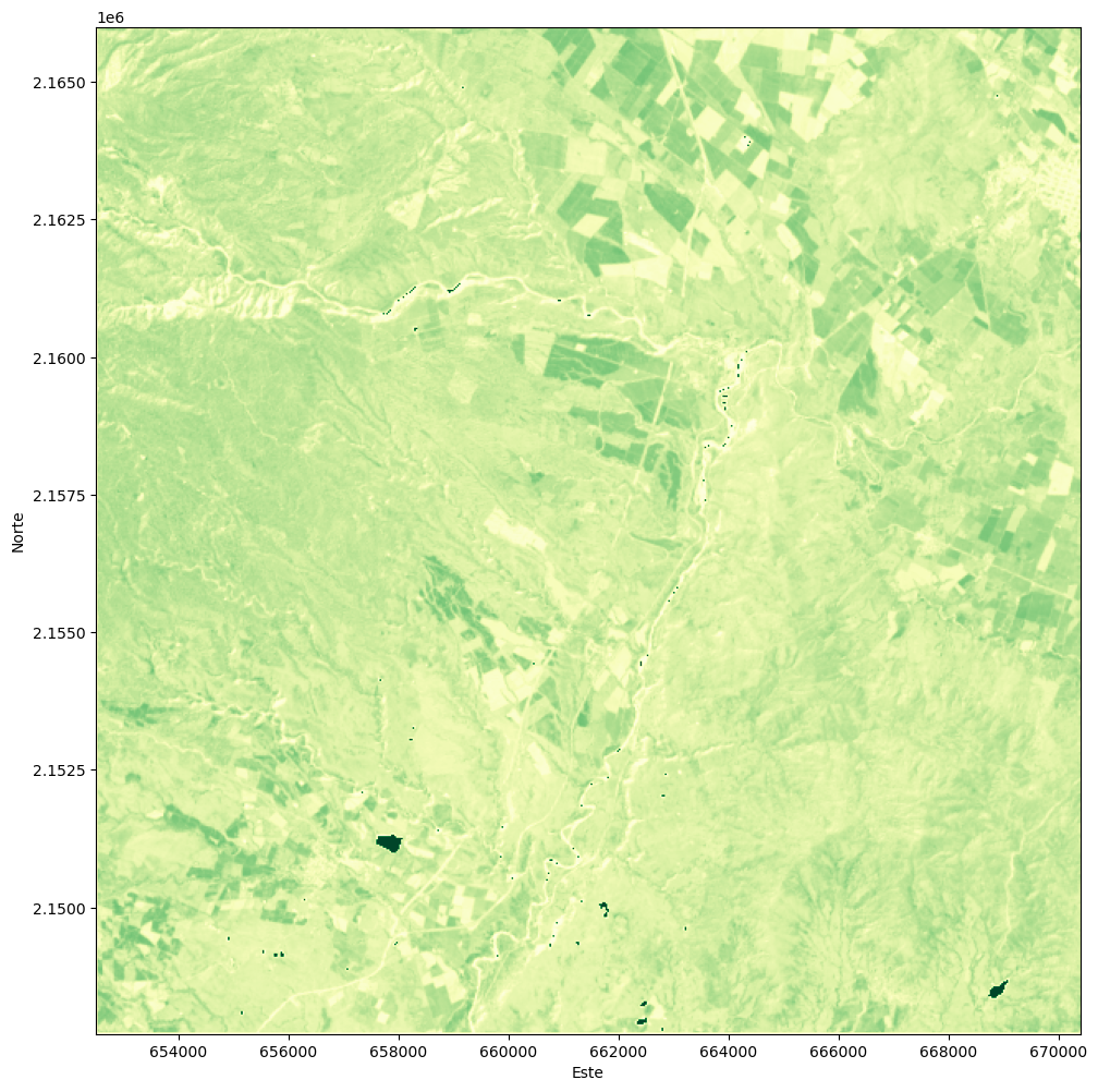

plotNDVIContour(path_NDVI_2014,'YlGn')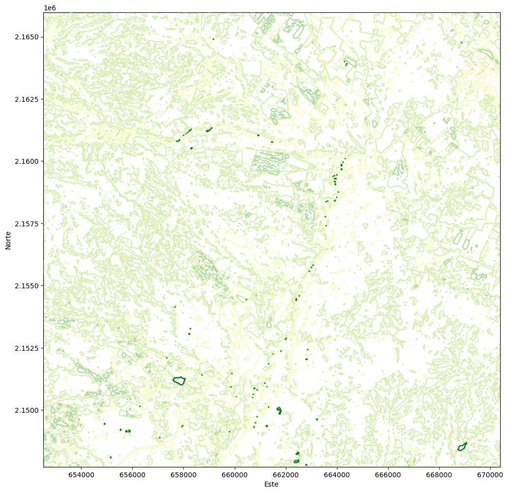

plotNDVI(path_NDVI_2019,'YlGn')

Create a land cover change image

We create a land cover change image based on the differences in NDVI from 2019 and 2014 imagery. The image will be stored as a separate file.

ndviChange = ndvi2019-ndvi2014
ndviChange = np.where((ndvi2014>-999) & (ndvi2019>-999),ndviChange,-999)
ndviChange

array([[ 0.        ,  0.03547079,  0.03795126, ...,  0.03159038,
         0.03800274,  0.02669263],
       [ 0.        ,  0.03765402,  0.05892348, ..., -0.00586917,
         0.01892243,  0.0195063 ],
       [ 0.        ,  0.03218401,  0.03739506, ..., -0.06377307,
        -0.0306757 ,  0.03894268],
       ...,
       [ 0.        , -0.01659706,  0.01140219, ...,  0.00272184,
         0.02552676,  0.06663901],
       [ 0.        ,  0.00599447, -0.00407705, ...,  0.05750174,
         0.00467577,  0.08448431],
       [ 0.        ,  0.        ,  0.        , ...,  0.        ,
         0.        ,  0.        ]])

saveRaster(ndviChange.astype('float32'),path_NDVIChange_19_14,cols,rows,projection)

plotNDVI(path_NDVIChange_19_14,'Spectral')