Delimitación de redes hídricas a partir de un DEM raster con Python y Landlab - Tutorial

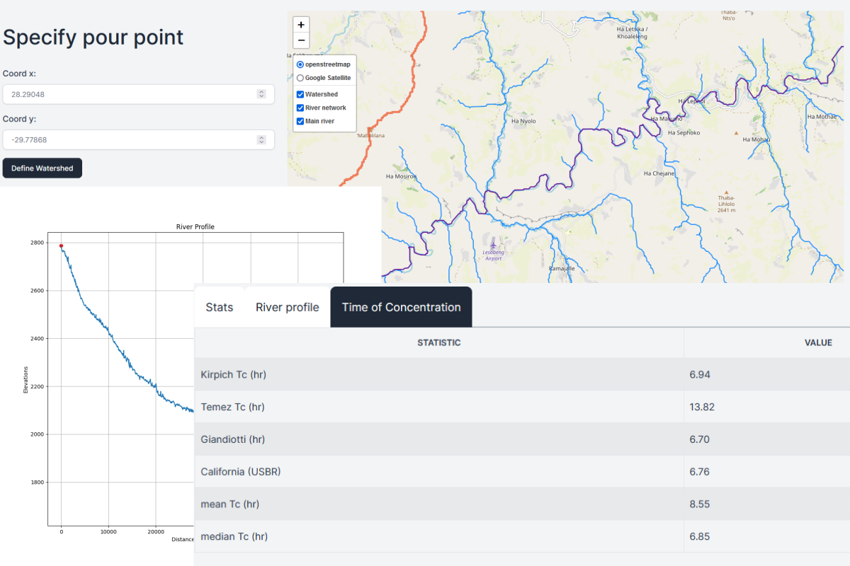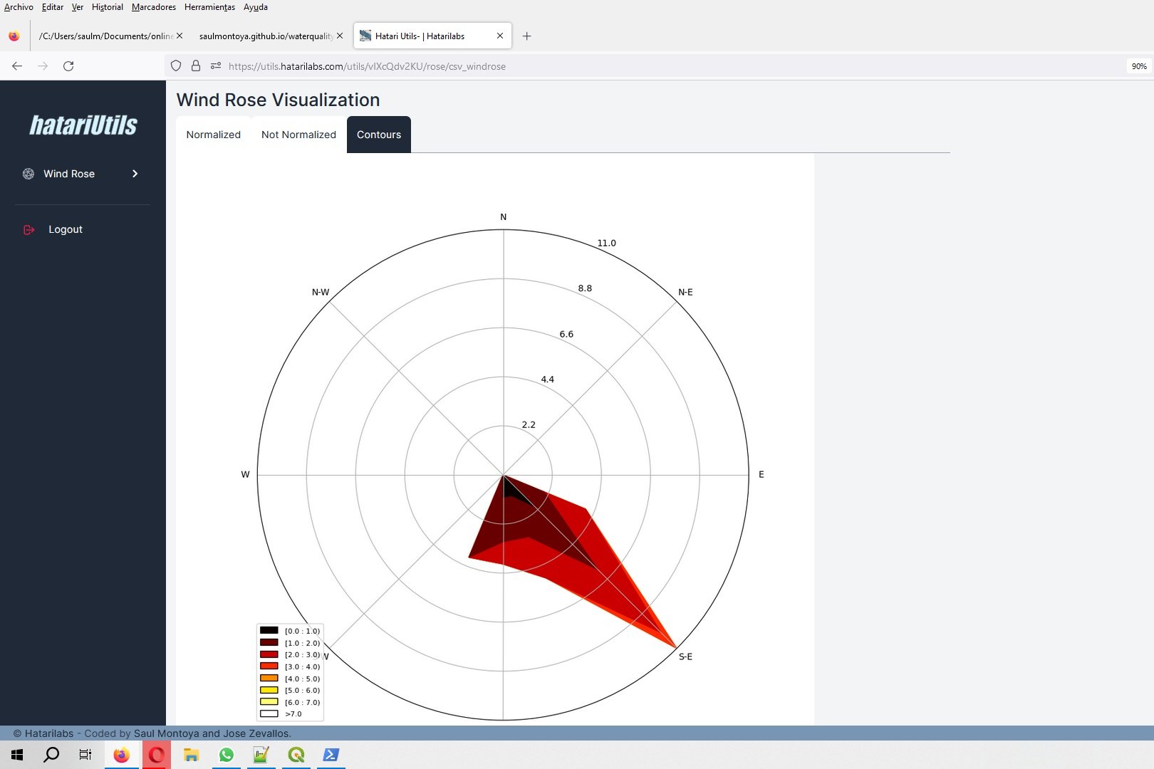
Nunca antes el proceso de delimitación de cuencas fue tan fácil. Ahora puedes delimitar cuencas y redes hídricas online con Hatari Utils:

utils.hatarilabs.com

Conoce más en este enlace:

gidahatari.com/ih-es/delimitacin-online-de-cuencas-y-redes-hdricas-con-hatari-utils-tutorial

En función de los diversos componentes de Landlab junto con otros paquetes de Python se pueden establecer algunos procedimientos para extraer redes de flujo únicas o múltiples de un ráster de modelo de elevación digital (DEM) y exportarlas como formatos de datos espaciales vectoriales como ESRI shapefiles o representarlos en Jupyter Lab .

Partes del tutorial:

• Abrir un archivo ráster y crear un Landlab ModelGrid

• Cálculo de la acumulación de flujo y relleno las depresiones

• Definición de canales con umbral de área de drenaje definido

Tutorial

Datos de entrada

Puede descargar los datos de entrada desde este enlace.

Código

# import generic packages
import numpy as np
from matplotlib import pyplot as plt

# import geospatial packages
import rasterio
from rasterio.plot import show
from shapely.geometry import LineString
import geopandas as gpd

# import landlab components
from landlab import RasterModelGrid, imshow_grid
from landlab.components import (
    DepressionFinderAndRouter,
    FlowAccumulator,
    ChannelProfiler,
)

# Open raster image 
rasterObj = rasterio.open('../rst/ASTGTM_NAD83_12N.tif')
show(rasterObj)

#extract array from raster
elevArray = rasterObj.read(1)
plt.imshow(elevArray)

#show array values
elevArray

array([[2319, 2319, 2296, ..., 1373, 1373, 1373],
       [2325, 2325, 2309, ..., 1371, 1373, 1373],
       [2334, 2334, 2315, ..., 1375, 1374, 1375],
       ..., 
       [2307, 2306, 2307, ..., 1800, 1799, 1789],
       [2299, 2295, 2295, ..., 1800, 1799, 1789],
       [2282, 2281, 2295, ..., 1814, 1805, 1796]], dtype=int16)

#create grid from raster attributes
nrows = rasterObj.height  # number of raster cells on each side, initially 150
ncols = rasterObj.width
dxy = (rasterObj.transform.a,-rasterObj.transform.e)  # side length of a raster model cell, or resolution [m], initially 50

# define a landlab raster
mg = RasterModelGrid(shape=(nrows, ncols), 
                     xy_spacing=dxy,
                     xy_of_lower_left=(rasterObj.bounds[0],rasterObj.bounds[1]))

# show number of rows, cols and resolution
print(nrows, ncols, dxy)

488 877 (21.514978563283933, 30.461871721312313)

# create a dataset of zero values
zr = mg.add_zeros("topographic__elevation", at="node")

# apply cell elevation to defined arrray
zr += elevArray[::-1,:].ravel()

imshow_grid(mg, "topographic__elevation", shrink=0.5)

#clear empty values
mg.set_nodata_nodes_to_closed(zr, -9999)

#flow direction
fa = FlowAccumulator(mg, flow_director='D4')
fa.run_one_step()

#fill sinks
df = DepressionFinderAndRouter(mg)
df.map_depressions()

#plot corrected drainage area
fig = plt.figure(figsize=(12,6))
imshow_grid(mg, 'drainage_area', shrink=0.5)

#profile the channel networks
profiler = ChannelProfiler(
    mg,
    number_of_watersheds=5,
    minimum_channel_threshold=1000000,
    main_channel_only=False)

#run profiler
profiler.run_one_step()

#extract profile dict
profDict = profiler.data_structure

#create a geopandas dataframe to store the channel network
multiLineList = []
multiLineIndex = []

for disPoint in profDict.keys():
    segDict = profDict[disPoint]   
    for segItem in segDict.keys():   
        coordList = []      
        nodeArray = segDict[segItem]['ids']
        for node in nodeArray:
            coordList.append([mg.x_of_node[node],mg.y_of_node[node]])
        multiLine = LineString(coordList)
        multiLineList.append(multiLine)
        multiLineIndex.append(segItem)
colDict = {'nodeStart':[a[0] for a in multiLineIndex],
          'nodeEnd':[a[1] for a in multiLineIndex]}
gdf = gpd.GeoDataFrame(colDict,index=range(len(multiLineIndex)), crs='epsg:'+str(rasterObj.crs.to_epsg()), geometry=multiLineList)

#show resulting geodataframe
gdf.head()

	nodeStart	nodeEnd	geometry
0	264854	233330	LINESTRING (362247.471 5248767.789, 362268.986...
1	233330	206983	LINESTRING (363280.190 5247671.162, 363301.705...
2	233330	212344	LINESTRING (363280.190 5247671.162, 363301.705...
3	212344	195715	LINESTRING (364614.119 5246940.077, 364635.634...
4	212344	213229	LINESTRING (364614.119 5246940.077, 364635.634...

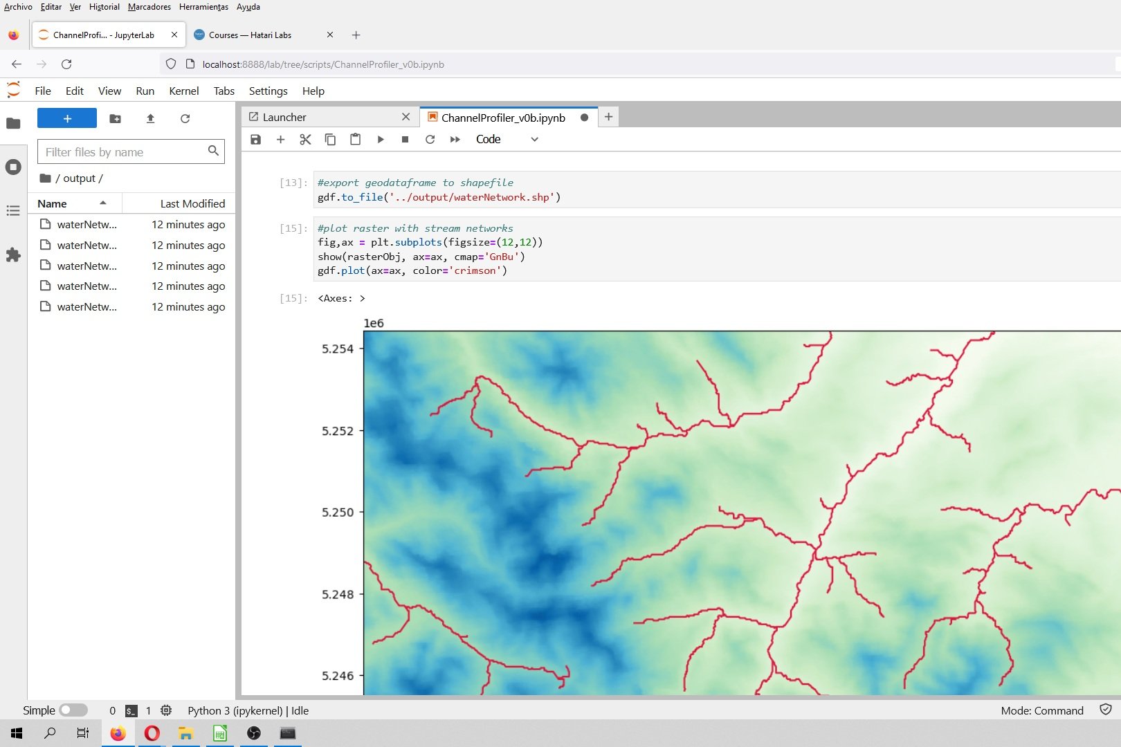
#export geodataframe to shapefile
gdf.to_file('../output/waterNetwork.shp')

#plot raster with stream networks
fig,ax = plt.subplots(figsize=(8,8))
show(rasterObj, ax=ax, cmap='GnBu')
gdf.plot(ax=ax, color='crimson')