Finalmente, una alternativa completa para la simulación de la intrusión salina en modelos de flujo de agua subterránea totalmente geoespaciales basados en software de código abierto. El modelo numérico se construyó en la plataforma Tupac Cloud con dos períodos de estrés y un tiempo total de simulación de 40 años. El proyecto se descarga desde Tupac Cloud y se ejecuta localmente con Anaconda donde se implementa en el script de Python el paquete BUY para el flujo de densidad variable junto con el modelo de transporte (GWT). También se desarrolla una representación gráfica de la cuadrícula, las condiciones de contorno y los resultados de los modelos de flujo y transporte en un entorno de Jupyter Lab.
Tutorial de referencia:
Tutorial
Datos de entrada
Puede descargar los datos de entrada desde este enlace.
Código
Este es el código en Python:
#import required packages
import flopy
import numpy as np
import matplotlib.pyplot as plt
import os
Open MF6 and explore packages
#open mf6 simulation and change folder path
simName = 'modflow'
simWs = os.path.abspath('../Model')
exeName = os.path.abspath('../bin/mf6.exe')
sim = flopy.mf6.MFSimulation.load('modflow',exe_name=exeName, sim_ws=simWs)
buySimWs = os.path.abspath('../modelBuy')
sim.set_sim_path(buySimWs)
#list sim packages
#sim.sim_package_list
#sim.write_simulation()#get groundwater flow model
gwf = sim.get_model()
#gwf#change folder of flow model
gwf.set_model_relative_path(os.path.abspath('../modelBuy'))# get model package list
gwf.get_package_list()Representation of model geometry
#open spatial discretization package
disv = gwf.get_package('DISV')
print(disv.top)
print(disv.botm)
#plot aerial plot
fig, ax = plt.subplots(figsize=(14,6))
mapview = flopy.plot.PlotMapView(model=gwf)
linecollection = mapview.plot_grid(lw=0.3)#plot cross sections
line = np.array([[200000,8800000], [214000,8800000]])
fig, ax = plt.subplots(figsize=(14,6))
crossview = flopy.plot.PlotCrossSection(model=gwf, line={"line": line})
crossview.plot_grid()Review boundary conditions
#General head boundary - GHB
fig, ax = plt.subplots(figsize=(14,6))
mapview = flopy.plot.PlotMapView(model=gwf)
linecollection = mapview.plot_grid(lw=0.1)
mapview.plot_bc('GHB_0')
#River - RIV
fig, ax = plt.subplots(figsize=(14,6))
mapview = flopy.plot.PlotMapView(model=gwf)
linecollection = mapview.plot_grid(lw=0.1)
mapview.plot_bc('RIV_0')fig, ax = plt.subplots(figsize=(14,6))
crossview = flopy.plot.PlotCrossSection(model=gwf, line={"line": line})
crossview.plot_grid()
crossview.plot_bc('RIV_0')#check output control
#gwf.get_package('OC')Create auxiliary variable and enable Buy package
#add auxiliary for ghb package
ghb = gwf.get_package('GHB')
ghbSpd = np.copy(ghb.stress_period_data.array)
ghb.auxiliary = 'CONCENTRATION'ghb.auxiliaryghbList = ghbSpd[0].tolist()
ghbList = [item + (0,) for item in ghbList]
ghbList[:5]ghbSpdDict = {}
ghbSpdDict[0] = ghbList
ghbSpdDict[1] = ghbListgwf.remove_package('GHB_0')ghb = flopy.mf6.modflow.ModflowGwfghb(gwf,auxiliary='CONCENTRATION', stress_period_data=ghbSpdDict)#define buy package
buyModName = 'modelBuy'
Csalt = 35.
Cfresh = 0.
densesalt = 1025.
densefresh = 1000.
denseslp = (densesalt - densefresh) / (Csalt - Cfresh)
pd = [(0, denseslp, 0., buyModName, 'CONCENTRATION')]
buy = flopy.mf6.ModflowGwfbuy(gwf, denseref=1000., nrhospecies=1,packagedata=pd)Define transport model
#create transport package
gwt = flopy.mf6.ModflowGwt(sim, modelname=buyModName)
#register solver for transport model
ims_gwt = flopy.mf6.ModflowIms(sim,linear_acceleration='BICGSTAB')
sim.register_ims_package(ims_gwt, [gwt.name])#define spatial discretization
gwtDisv = flopy.mf6.ModflowGwtdisv(gwt, nlay=disv.nlay.data,
ncpl=disv.ncpl.data,
nvert=disv.nvert.data,
top=disv.top.data,
botm=disv.botm.data,
vertices=disv.vertices.array.tolist(),
cell2d=disv.cell2d.array.tolist(),
)#define starting concentrations
strtConc = np.zeros((disv.nlay.data, disv.ncpl.data), dtype=np.float32)ghbList = ghb.stress_period_data.array[0].tolist()
ghbList[:5]for ghbItem in ghbList:
strtConc[:,ghbItem[0][1]] = 35
gwtIc = flopy.mf6.ModflowGwtic(gwt, strt=strtConc)fig = plt.figure(figsize=(12, 12))
ax = fig.add_subplot(1, 1, 1, aspect = 'equal')
mapview = flopy.plot.PlotMapView(model=gwf,layer = 1)
plot_array = mapview.plot_array(strtConc,masked_values=[-1e+30], cmap=plt.cm.summer)
plt.colorbar(plot_array, shrink=0.75,orientation='horizontal', pad=0.08, aspect=50)#define advection
adv = flopy.mf6.ModflowGwtadv(gwt, scheme='UPSTREAM')#define dispersion
#dsp = flopy.mf6.ModflowGwtdsp(gwt,diffc=0.707,alh=5,alv=5,ath1=2)
dsp = flopy.mf6.ModflowGwtdsp(gwt,alh=10,ath1=10)#define mobile storage and transfer
porosity = 0.30
sto = flopy.mf6.ModflowGwtmst(gwt, porosity=porosity)#define sink and source package
sourcerecarray = ['GHB_0','AUX','CONCENTRATION']
ssm = flopy.mf6.ModflowGwtssm(gwt, sources=sourcerecarray)#define constant concentration package
cncSp = []
for row in ghb.stress_period_data.array[0]:
cncSp.append([row[0],35])
cncSpd = {0:cncSp,1:cncSp}
cnc = flopy.mf6.ModflowGwtcnc(gwt,stress_period_data=cncSpd)cnc.plot(mflay=0, lw=0.1, figsize=(12,12))#define output control
oc = flopy.mf6.ModflowGwtoc(gwt,
concentration_filerecord=buyModName+'.ucn',
saverecord=[('CONCENTRATION', 'ALL')])Define model exchange, write and run model
#define model flow and transport exchange
name = 'modelExchange'
gwfgwt = flopy.mf6.ModflowGwfgwt(sim, exgtype='GWF6-GWT6',
                                 exgmnamea=gwf.name, exgmnameb=buyModName,
                                 filename='{}.gwfgwt'.format(name))
#write simulation and run simulation
sim.write_simulation()
#sim.run_simulation()#fix tupacModel.nam
sim.run_simulation()Explore the head results
#import heads
headObj = flopy.utils.HeadFile(os.path.join(buySimWs,'tupacModel.hds'))
tsList = headObj.get_kstpkper()
tsList
### Review the flow model
fig = plt.figure(figsize=(12, 12))
ax = fig.add_subplot(1, 1, 1, aspect = 'equal')
mapview = flopy.plot.PlotMapView(model=gwf,layer = 3)
ts = (0, 0)
tempHead = headObj.get_data(kstpkper=ts)
tempHead[tempHead==gwf.hdry] = np.nan
plot_array = mapview.plot_array(tempHead,masked_values=[-1e+30], cmap=plt.cm.Blues)
plt.colorbar(plot_array, shrink=0.75,orientation='horizontal', pad=0.08, aspect=50)Explore the concentration results
#import heads and concentrations
concObj = flopy.utils.HeadFile(os.path.join(buySimWs,buyModName+'.ucn'), text='CONCENTRATION')
#define time series and stress period to plot
ts = (3, 1)
#get concentrations for the time step
tempConc = concObj.get_data(kstpkper=ts)### Review the flow model
fig = plt.figure(figsize=(12, 12))
ax = fig.add_subplot(1, 1, 1, aspect = 'equal')
mapview = flopy.plot.PlotMapView(model=gwf,layer = 2)
plot_array = mapview.plot_array(tempConc,masked_values=[-1e+30], cmap=plt.cm.summer)
plt.colorbar(plot_array, shrink=0.75,orientation='horizontal', pad=0.08, aspect=50)### Zoom to intrusion
fig = plt.figure(figsize=(12, 12))
ax = fig.add_subplot(1, 1, 1, aspect = 'equal')
mapview = flopy.plot.PlotMapView(model=gwf,layer = 2)
plot_array = mapview.plot_array(tempConc,masked_values=[-1e+30], cmap=plt.cm.summer)
plt.colorbar(plot_array, shrink=0.75,orientation='horizontal', pad=0.08, aspect=50)
ax.set_xlim(200000,206000)
ax.set_ylim(8798000,8803000)#plot heads on line
tempHead = headObj.get_data(kstpkper=ts)
fig, ax = plt.subplots(figsize=(18,6))
line = np.array([[200000,8801800], [214000,8803000]])
crossview = flopy.plot.PlotCrossSection(model=gwf, line={"line": line})
crossview.plot_grid(alpha=0.25)
strtArray = crossview.plot_array(tempHead, masked_values=[1e30])
wtElev = []
for col in range(tempHead.shape[2]):
colArray = tempHead[:,0,col]
wtElev.append(colArray[colArray != 1e30][0])
wt = crossview.plot_surface(tempHead, color="blue", lw=2)
#wtLine = plt.plot(gwf.modelgrid.xycenters[0],wtElev,c='crimson')
cb = plt.colorbar(strtArray, shrink=0.5)#plot concentrations on row 5
fig, ax = plt.subplots(figsize=(18,6))
crossview = flopy.plot.PlotCrossSection(model=gwf, line={"line": line})
crossview.plot_grid(alpha=0.25)
strtArray = crossview.plot_array(tempConc, masked_values=[1e30], cmap=plt.cm.summer)
cb = plt.colorbar(strtArray, shrink=0.5)#plot concentrations on line - zoom
fig, ax = plt.subplots(figsize=(18,6))
crossview = flopy.plot.PlotCrossSection(model=gwf, line={"line": line})
crossview.plot_grid(alpha=0.25)
strtArray = crossview.plot_array(tempConc, masked_values=[1e30], cmap=plt.cm.summer)
cb = plt.colorbar(strtArray, shrink=0.5)
ax.set_xlim(0,1500)