Como importar un modelo geológico de Leapfrog a Model Muse con Python - Tutorial

Tener un modelo geológico puede mejorar los modelos numéricos, ya que permite representar con mayor precisión la distribución potencial de parámetros hidráulicos en dirección horizontal y vertical. El proceso de implementar/incorporar un modelo geológico en un modelo Modflow es un desafío debido a las restricciones en software propietario y herramientas espaciales.

Hemos realizado un tutorial que muestra todo el procedimiento para insertar un modelo geológico en un modelo de aguas subterráneas MODFLOW-NWT con scripts en Python, Pyvista y otros. El código extrae los centroides de celda del modelo de Modflow y luego compara su posición con las diferentes unidades geológicas exportadas de Leapfrog a Vtk. Una vez identificada la litología correspondiente de la celda, se asigna un parámetro hidráulico. El tutorial funciona a partir de Vtks de un modelo geológico hecho en Leapfrog, pero puede funcionar con cualquier Vtk.

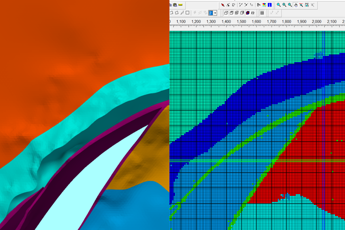
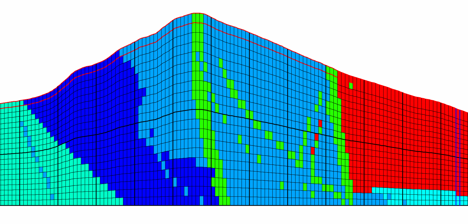
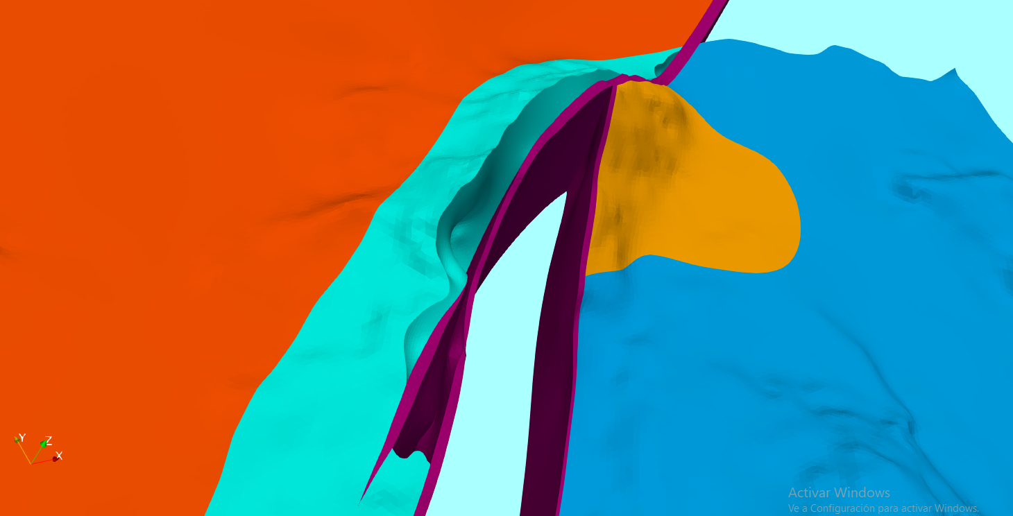
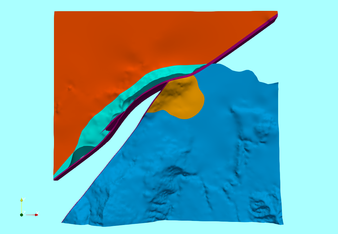
Este tutorial requiere los archivos Vtk generados de modelos geológicos en Leapfrog que se muestran en este tutorial:

gidahatari.com/ih-es/como-convertir-unidades-geolgicas-de-leapfrog-msh-a-vtk-con-python-y-gemgis-tutorial

Capturas de pantalla

Tutorial

Código

# Import required models
import os
import flopy
import numpy as np
import pyvista as pv
import matplotlib.pyplot as plt
from matplotlib.colors import LogNorm

# Open modflow model 
modWs = '../Model/'
mf = flopy.modflow.Modflow.load('Model1.nam',model_ws=modWs)

C:\Users\saulm\anaconda3\Lib\site-packages\flopy\mbase.py:85: UserWarning: The program mf2005 does not exist or is not executable.
  warn(

# Set coord info for spatial query
# From Model1.dis
# Lower left corner: (1444500, 5246300)
mf.modelgrid.set_coord_info(1444500, 5246300)

# Convert the cell centers into a flattened numpy array
xyzCellList = mf.modelgrid.xyzcellcenters
# for x,y,z
xArray = np.tile(xyzCellList[0],(mf.modelgrid.nlay,1)).flatten()
yArray = np.tile(xyzCellList[1],(mf.modelgrid.nlay,1)).flatten()
zArray = xyzCellList[2].flatten()
# stack x, y, z columns
xyzCells = np.column_stack([xArray,yArray,zArray])
xyzCells.shape

(3040000, 3)

# Transform xyz list to a Pyvista polydata
xyzPoly = pv.PolyData(xyzCells)
xyzPoly

PolyData	Information
N Cells	3040000
N Points	3040000
N Strips	0
X Bounds	1.445e+06, 1.448e+06
Y Bounds	5.246e+06, 5.250e+06
Z Bounds	-1.467e+02, 7.011e+02
N Arrays	0

---

Working with Vtks and appliying spatial queries

# Get all vtks from directory and assign a correlative id
litoDict = [{'unit':unit,'vtk':vtk} for unit, vtk in enumerate(os.listdir('../Vtk')) if vtk.endswith('.vtk')]
#litoDict = litoDict[:1]
litoDict

[{'unit': 0, 'vtk': 'brecciaMsh.vtk'},
 {'unit': 1, 'vtk': 'dykeMsh.vtk'},
 {'unit': 2, 'vtk': 'granoMsh.vtk'},
 {'unit': 3, 'vtk': 'marbleMsh.vtk'},
 {'unit': 4, 'vtk': 'sandMsh.vtk'}]

#create a list with a default lito code (5)
compLitoList = [5 for x in range(mf.modelgrid.size)]
len(compLitoList)

3040000

#we iterate over all litos to assign the lito values
for lito in litoDict:
    #open the vtk file for the selected lito
    tempVtk = pv.read('../Vtk/'+lito['vtk'])
    #check if points are inside the vtk object
    checkPoints = xyzPoly.select_enclosed_points(tempVtk)
    #get only the inside points
    insidePointsIndex = np.nonzero(checkPoints['SelectedPoints']==1)[0]
    #assign the lito code to the compound lito list
    for pointIndex in insidePointsIndex:
        compLitoList[pointIndex] = lito['unit']

#now we can have a look of the lito at model grid scale
compLitoArray = np.array(compLitoList)
compLitoArray = np.reshape(compLitoArray,[mf.modelgrid.nlay,
                                          mf.modelgrid.nrow,
                                          mf.modelgrid.ncol])

#show array distribution
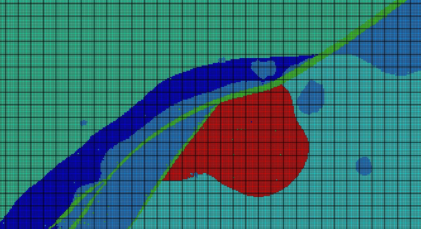
plt.imshow(compLitoArray[5])

<matplotlib.image.AxesImage at 0x1fb4cdcedd0>

---

Applying parameters to model

# Open the modflow package that stores hydraulic parameters
lpf = mf.get_package('LPF')
hkArray= np.copy(lpf.hk.array)
hkArray.shape

(20, 380, 400)

# Define the k values for every lito code
kDict = {
    0:6.5e-4,
    1:3.6e-6,
    2:2.5e-7,
    3:1.6e-8,
    4:5.4e-7,
    5:5.8e-8
}

# ov
for lay in range(mf.modelgrid.nlay):
    for row in range(mf.modelgrid.nrow):
        for col in range(mf.modelgrid.ncol):
            litoCode = compLitoArray[lay,row,col]
            hkArray[lay,row,col] = kDict[litoCode]

#show applied values
plt.imshow(hkArray[5], norm=LogNorm())
plt.show()

# Change working directory to store modified model
mf.change_model_ws('../workingModel/')
# Apply k values as an array
lpf.hk = hkArray

# Show applied values
lpf.hk.plot(mflay=10, norm=LogNorm())
plt.show()

mf.write_input()

Datos de entrada

Puede descargar los datos de entrada desde este enlace.