La calidad de un modelo de aguas subterráneas como herramienta para la gestión sostenible de nuestros recursos hídricos subterráneos no depende de la calidad de los datos de entrada, la precisión de la calibración, sino también de la visualización de los datos de salida y el análisis del balance hídrico. Hay varias opciones para exportar contornos desde MODFLOW GUIs como Model Muse, sin embargo, al analizar varios períodos de requerimiento (stress periods), los pasos pueden llevar mucho tiempo, por lo que un script de Python sería útil para exportar cargas hidráulicas o niveles freáticos como shapefiles.
Para realizar este tutorial necesita un entorno de Conda con librerías geospaciales. Instale el entorno siguiendo este enlace: gidahatari.com/ih-es/como-instalar-python-geopandas-en-windows-bajo-un-entorno-en-conda-tutorial
Video
Código
#!pip install flopy
import os
import numpy as np
import matplotlib.pyplot as plt
import flopy
#import shapefile as sf #in case you dont have it, form anaconda prompt: pip install pyshp
from flopy.utils.gridgen import Gridgen
from flopy.utils.reference import SpatialReference
import pandas as pd
from scipy.interpolate import griddata
modelname='regionalModel1'
model_ws= '../Model/'
mf = flopy.modflow.Modflow.load(modelname+'.nam', version="mfnwt" ,model_ws=model_ws)# Lower left corner: (611991.514073899, 8354016.396838)
# Grid angle (in degrees counterclockwise): -24
xll = 611991.514073899
yll = 8354016.396838
epsg = 32718
rotation = -24
mf.modelgrid.set_coord_info(xoff=xll, yoff=yll, angrot=rotation,epsg=2236)fig = plt.figure(figsize=(8,8))
ax = fig.add_subplot(1, 1, 1, aspect='equal')
modelmap = flopy.plot.PlotMapView(model=mf)
linecollection = modelmap.plot_grid(linewidth=0.5, color='royalblue')
#import head data
mfheads = flopy.utils.HeadFile('../Model/'+modelname+'.bhd',text='head')
mftimes = mfheads.get_times()
mftimes[:3][1.0]# find shape
head = mfheads.get_data()
shape = head.shape
shape(5, 138, 75)#create a array an empty array
drnArray = np.zeros(shape[1:])
drnArray[:] = np.NaN
#fill the values for the water table
for row in range(shape[1]):
for col in range(shape[2]):
drnValues = head[:,row,col]
for value in drnValues:
if value > 0:
drnArray[row,col]=value
break
plt.imshow(drnArray)<matplotlib.image.AxesImage at 0x1b54ae10970>
#get min and max head for contour levels
headMin = head[head>-1.e+20].min()
headMax = head[head>-1.e+20].max()
print(headMin,headMax)
3431.9033 4439.018#define contours levels
levels = np.linspace(headMin,headMax,25)
levelsarray([3431.90332031, 3473.86643473, 3515.82954915, 3557.79266357,
3599.75577799, 3641.71889242, 3683.68200684, 3725.64512126,
3767.60823568, 3809.5713501 , 3851.53446452, 3893.49757894,
3935.46069336, 3977.42380778, 4019.3869222 , 4061.35003662,
4103.31315104, 4145.27626546, 4187.23937988, 4229.2024943 ,
4271.16560872, 4313.12872314, 4355.09183757, 4397.05495199,
4439.01806641])# Plot the heads for a defined layer and boundary conditions
fig = plt.figure(figsize=(36, 24))
ax = fig.add_subplot(1, 1, 1, aspect='equal')
modelmap = flopy.plot.PlotMapView(model=mf)
contour = modelmap.contour_array(drnArray,ax=ax, levels=levels)
cellhead = modelmap.plot_array(drnArray,ax=ax, cmap='Blues', alpha=0.2)
ax.clabel(contour)
ax.grid()
plt.tight_layout()
import fiona

# define schema
schema = {
    'geometry':'LineString',
    'properties':[('waterTable','float')]
}
#open a fiona object
polyShp = fiona.open('../Shps/waterTable_v1.shp', mode='w', driver='ESRI Shapefile',
          schema = schema, crs = "EPSG:32718")

for index, c in enumerate(contour.allsegs):
    try:
    #save record and close shapefile
        tupleList = [(a[0],a[1]) for a in c[0]]
        #print(tupleList)
        rowDict = {
            'geometry' : {'type':'LineString',
                             'coordinates': tupleList}, #Here the xyList is in brackets
            'properties': {'waterTable' : contour.cvalues[index]},
            }
        polyShp.write(rowDict)
    except IndexError:
        pass

#close fiona object
polyShp.close()
Datos de entrada
Puede descargar los datos de entrada desde este enlace.