El método de diferencias finitas, así como cualquier otro método de discretización, permite la conceptualización de un medio geológico en céldas u otros volúmenes. Los modelos geológicos vienen en diversos formatos en formato binario o de texto y necesitan ser "traducidos" a la estructura grillada de un modelo de agua subterránea.
Este tutorial tiene un ejemplo aplicado de la implementación de un modelo geológico 3D desde una red neuronal a un modelo de agua subterránea con discretización horizontal y espesor de capa determinados. El tutorial cubre todos los pasos para la construcción de la geometría de un modelo y la determinación de unidades hidrogeológicas con scripts en Python, Flopy y otras bibliotecas. Las comparaciones del modelo geológico original y traducido se realizaron como diagramas de Matplotlib y archivos Vtk en Paraview.
Video
Código
Este es el código principal desarrollado en este tutorial:
import os
import flopy
import numpy as np
import pandas as pd
import matplotlib.pyplot as plt
from flopy.utils.reference import SpatialReference
from scipy.interpolate import griddata
from shapely.geometry import Polygon
flopy is installed in /home/wk-gida1/.local/lib/python3.7/site-packages/flopyDefinition of area of interest and output grid refinement
xMin = 540000
xMax = 560000
yMin = 4820000
yMax = 4840000
aoiGeom = Polygon(((xMin,yMin),(xMax,yMin),(xMax,yMax),(xMin,yMax),(xMin,yMin)))
cellH = 250
vertexCols = np.arange(xMin,xMax+1,cellH)
vertexRows = np.arange(yMax,yMin-1,-cellH)
cellCols = (vertexCols[1:]+vertexCols[:-1])/2
cellRows = (vertexRows[1:]+vertexRows[:-1])/2
nCols = cellCols.shape[0]
nRows = cellRows.shape[0]Creation of a model topo
# Open well location:
wellLoc = pd.read_csv("../inputData/TV-HFM_Wells_1Location_Wgs11N.csv",index_col=0)
wellLoc.head()| Easting | Northing | Altitude_ft | EastingUTM | NorthingUTM | Elevation_m | |
|---|---|---|---|---|---|---|
| Bore | ||||||
| A. Isaac | 2333140.95 | 1372225.65 | 3204.0 | 575546.628834 | 4.820355e+06 | 976.57920 |
| A. Woodbridge | 2321747.00 | 1360096.95 | 2967.2 | 564600.366582 | 4.807827e+06 | 904.40256 |
| A.D. Watkins | 2315440.16 | 1342141.86 | 3168.3 | 558944.843404 | 4.789664e+06 | 965.69784 |
| A.L. Clark; 1 | 2276526.30 | 1364860.74 | 2279.1 | 519259.006159 | 4.810959e+06 | 694.66968 |
| A.L. Clark; 2 | 2342620.87 | 1362980.46 | 3848.6 | 585351.150270 | 4.811460e+06 | 1173.05328 |
points = wellLoc[['EastingUTM','NorthingUTM']].values
values = wellLoc['Elevation_m'].values
grid_x = np.tile(cellCols,(nRows,1))
grid_y = np.tile(cellRows,(nCols,1)).T
mtop = griddata(points, values, (grid_x, grid_y), method='linear')
print(mtop[:5,:5])
print(mtop.max())
[[769.26668708 769.93247791 770.59826874 771.26405958 771.92985041]
[767.33963938 768.00543022 768.67122105 769.33701188 770.00280272]
[765.41259169 766.07838252 766.74417336 767.40996419 768.07575502]
[763.70469671 764.15133483 764.81712566 765.4829165 766.14870733]
[762.36605826 762.22428714 762.89007797 763.55586881 764.22165964]]
930.0534171904137plt.imshow(mtop)<matplotlib.image.AxesImage at 0x7f3fe0c3ddd0>
Modflow model object and DIS package
modelname='Model1'
model_ws= '../Model'
mf = flopy.modflow.Modflow(modelname, exe_name="../../../Solvers/mfnwt", version="mfnwt",model_ws=model_ws)

#Definition of MODFLOW NWT Solver
nwt = flopy.modflow.ModflowNwt(mf ,maxiterout=250,linmeth=2,headtol=0.01,Continue=True)

# setting up the vertical discretization and model bottom elevation
nLays = 5
AcuifInf_Bottom = 500

zbot = np.zeros((nLays,nRows,nCols))
zbot[0,:,:] = AcuifInf_Bottom + (0.88 * (mtop - AcuifInf_Bottom))
zbot[1,:,:] = AcuifInf_Bottom + (0.76 * (mtop - AcuifInf_Bottom))
zbot[2,:,:] = AcuifInf_Bottom + (0.6 * (mtop - AcuifInf_Bottom))
zbot[3,:,:] = AcuifInf_Bottom + (0.4 * (mtop - AcuifInf_Bottom))
zbot[4,:,:] = AcuifInf_Bottom

# Dis package
dis = flopy.modflow.ModflowDis(mf, nlay=nLays,
                               nrow=nRows,ncol=nCols,
                               delr=cellH,delc=cellH,
                               top=mtop,botm=zbot,
                               itmuni=1.,nper=1,perlen=1,nstp=1,steady=True)

mf.modelgrid.set_coord_info(xoff=xMin, yoff=yMin, angrot=0,epsg=32611)

fig = plt.figure(figsize=(12,8))
ax = fig.add_subplot(1, 1, 1, aspect='equal')
modelmap = flopy.plot.PlotMapView(model=mf)
linecollection = modelmap.plot_grid(linewidth=0.5, color='royalblue')
fig = plt.figure(figsize=(20, 6))
ax = fig.add_subplot(1, 1, 1)
modelxsect = flopy.plot.PlotCrossSection(model=mf, line={'Column': 0})
linecollection = modelxsect.plot_grid()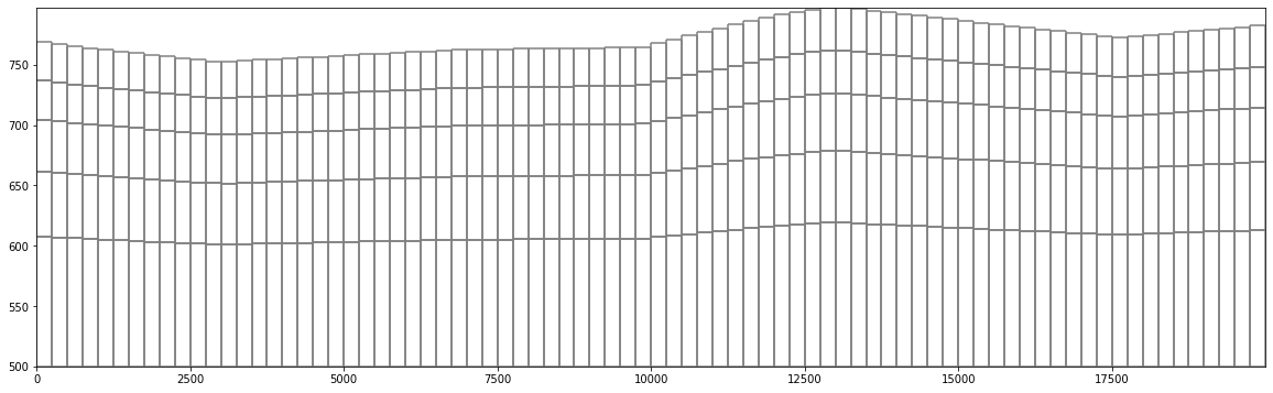
Apply the lithological model and UPW package
#open the 3D lithological model as x,y,z,lito list
zVerts = mf.modelgrid.zvertices
litoList = np.load("../processedData/litoListXYZL.npy")
print(litoList[:5])
print(litoList[-1])
print(litoList.shape)

#initialization of model hydraulic conductivity
hK = np.zeros([nLays,nRows,nCols])

[[5.4010e+05 4.8399e+06 8.2900e+02 3.0000e+00]
 [5.4030e+05 4.8399e+06 8.2900e+02 3.0000e+00]
 [5.4050e+05 4.8399e+06 8.2900e+02 3.0000e+00]
 [5.4070e+05 4.8399e+06 8.2900e+02 3.0000e+00]
 [5.4090e+05 4.8399e+06 8.2900e+02 3.0000e+00]]
[5.5990e+05 4.8201e+06 5.4900e+02 3.0000e+00]
(150000, 4)

import statistics, copy
i=0
for lay in range(nLays):
    for row in range(nRows):
        for col in range(nCols):
            cellXMin = vertexCols[col]
            cellXMax = vertexCols[col+1]
            cellYMin = vertexRows[row+1]
            cellYMax = vertexRows[row]
            cellZMin = zVerts[lay+1,row,col]
            cellZMax = zVerts[lay,row,col]

            litoAux = copy.copy(litoList)
            litoAux = litoAux[litoAux[:,0] >= cellXMin]
            litoAux = litoAux[litoAux[:,0] < cellXMax]
            litoAux = litoAux[litoAux[:,1] >= cellYMin]
            litoAux = litoAux[litoAux[:,1] < cellYMax]
            litoAux = litoAux[litoAux[:,2] >= cellZMin]
            litoAux = litoAux[litoAux[:,2] < cellZMax]


            litoValues = list(litoAux[:,3])

            if len(litoValues)>0:
                try:
                    litoMode = statistics.mode(litoValues)
                except statistics.StatisticsError:
                    litoMode = max(litoValues)
            else:
                print("No values found %s"%str([lay,row,col]))
                litoMode = 1

            if i%5000==0:
                print(lay,row,col)
                print(litoValues)
                print(litoMode)
            i+=1

            hK[lay,row,col]=litoMode

0 0 0
[2.0, 2.0]
2.0
No values found [0, 0, 70]
No values found [0, 0, 71]
No values found [0, 0, 72]
No values found [0, 0, 73]
No values found [0, 0, 74]
No values found [0, 0, 75]
No values found [0, 0, 76]
No values found [0, 0, 77]
No values found [0, 0, 78]
No values found [0, 0, 79]
No values found [0, 1, 71]
No values found [0, 1, 72]
No values found [0, 1, 73]
No values found [0, 1, 74]
No values found [0, 1, 75]
No values found [0, 1, 76]
No values found [0, 1, 77]
No values found [0, 1, 78]
No values found [0, 1, 79]
No values found [0, 2, 72]
No values found [0, 2, 73]
No values found [0, 2, 74]
No values found [0, 2, 75]
No values found [0, 2, 76]
No values found [0, 2, 77]
No values found [0, 2, 78]
No values found [0, 2, 79]
No values found [0, 3, 73]
No values found [0, 3, 74]
No values found [0, 3, 75]
No values found [0, 3, 76]
No values found [0, 3, 77]
No values found [0, 3, 78]
No values found [0, 3, 79]
No values found [0, 4, 74]
No values found [0, 4, 75]
No values found [0, 4, 76]
No values found [0, 4, 77]
No values found [0, 4, 78]
No values found [0, 4, 79]
No values found [0, 5, 75]
No values found [0, 5, 76]
No values found [0, 5, 77]
No values found [0, 5, 78]
No values found [0, 5, 79]
No values found [0, 6, 76]
No values found [0, 6, 77]
No values found [0, 6, 78]
No values found [0, 6, 79]
No values found [0, 7, 77]
No values found [0, 7, 78]
No values found [0, 7, 79]
No values found [0, 8, 78]
No values found [0, 8, 79]
No values found [0, 9, 79]
0 62 40
[1.0, 1.0]
1.0
No values found [0, 76, 77]
No values found [0, 76, 78]
No values found [0, 76, 79]
No values found [0, 77, 73]
No values found [0, 77, 74]
No values found [0, 77, 75]
No values found [0, 77, 76]
No values found [0, 77, 77]
No values found [0, 77, 78]
No values found [0, 77, 79]
No values found [0, 78, 72]
No values found [0, 78, 73]
No values found [0, 78, 74]
No values found [0, 78, 75]
No values found [0, 78, 76]
No values found [0, 78, 77]
No values found [0, 78, 78]
No values found [0, 78, 79]
No values found [0, 79, 71]
No values found [0, 79, 72]
No values found [0, 79, 73]
No values found [0, 79, 74]
No values found [0, 79, 75]
No values found [0, 79, 76]
No values found [0, 79, 77]
No values found [0, 79, 78]
No values found [0, 79, 79]
1 45 0
[2.0, 2.0, 2.0, 2.0]
2.0
2 27 40
[1.0, 1.0]
1.0
3 10 0
[2.0, 2.0, 2.0]
2.0
3 72 40
[3.0, 3.0, 3.0, 3.0]
3.0
4 55 0
[3.0, 2.0, 2.0, 2.0]
2.0

# Definition of layer type, the first two layers are convertible
laytyp = [1,1,0,0,0]
upw = flopy.modflow.ModflowUpw(mf, laytyp = laytyp, hk=hK, vka=hK, ss=5e-06, sy=0.12) #vka= Kx,

fig = plt.figure(figsize=(20, 3))
ax = fig.add_subplot(1, 1, 1)
modelxsect = flopy.plot.PlotCrossSection(model=mf, line={'Row': 0})
linecollection = modelxsect.plot_grid()
modelxsect.plot_array(hK)

<matplotlib.collections.PatchCollection at 0x7f3fdfc97f50>
mf.write_input()Datos de entrada
Puede descargar los datos de entrada desde este enlace.