Completación de Datos Faltantes de Precipitación con Python y Scikit-Learn - Tutorial

La evaluación de procesos de precipitación, escorrentía, enrutamiento, así como la infiltración requieren de datos de precipitación, caudal, temperatura y radiación a escala diaria. Los datos requeridos por los modelos hidrológicos deben ser confiables y estar completos en el periodo de estudio. Muchas veces los datos de estaciones de precipitación, aforo, entre otros se presentan incompletos en varias partes siendo posible su completación mediante mediante el uso de algoritmos como Scikit-Learn en Python3.

Este tutorial tiene por objetivo mostrar el procedimiento de la ejecución de un script para completar datos de precipitación proveído de dos estaciones cercanas. El script se ejecutará en Python 3.9 en el entorno de Anaconda Prompt.

Tutorial

Código

#!pip install sklearn
import pandas as pd
import numpy as np
import matplotlib.pyplot as plt
from sklearn.preprocessing import StandardScaler
from sklearn.neural_network import MLPRegressor

precipStations =  pd.read_csv('../Data/Est1_Est2_Est3.csv',index_col=0,parse_dates=True)
precipStations.head()

	Est1	Est2	Est3
Fecha
2014-07-25	0.0	NaN	0.0
2014-07-26	0.6	NaN	0.0
2014-07-27	0.0	NaN	0.0
2014-07-28	0.0	NaN	0.0
2014-07-29	0.2	NaN	0.2

fig, axs=plt.subplots(3,1,figsize=(12,8),sharex=True,sharey=True)
axs[0].plot(precipStations.index,precipStations['Est1'],label='Est1')
axs[0].legend()
axs[1].plot(precipStations.index,precipStations['Est2'],label='Est2')
axs[1].legend()
axs[2].plot(precipStations.index,precipStations['Est3'],label='Est3')
axs[2].legend()
plt.xticks(rotation='vertical')
plt.show()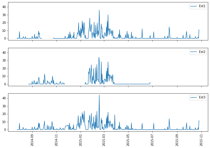

precipNotNan = precipStations.dropna()
precipNotNan

	Est1	Est2	Est3
Fecha
2014-08-23	0.0	0.0	0.0
2014-08-24	0.0	0.0	0.0
2014-08-25	0.0	0.0	0.0
2014-08-26	0.0	0.0	0.0
2014-08-27	0.0	0.0	0.0
...	...	...	...
2015-06-21	0.0	0.0	0.0
2015-06-22	0.0	0.0	0.0
2015-06-23	0.0	0.0	0.0
2015-06-24	0.0	0.0	0.0
2015-06-25	3.8	2.2	0.0

229 rows × 3 columns

xTrain = precipNotNan[['Est1','Est3']]
yTrain = precipNotNan[['Est2']].values.flatten()

print(xTrain[:10])
print(yTrain[:10])

Est1  Est3
Fecha                 
2014-08-23   0.0   0.0
2014-08-24   0.0   0.0
2014-08-25   0.0   0.0
2014-08-26   0.0   0.0
2014-08-27   0.0   0.0
2014-08-28   0.0   0.0
2014-08-29   0.0   0.0
2014-08-30   0.0   0.0
2014-08-31   0.0   0.0
2014-09-01   2.8   3.4
[0.  0.  0.  0.  0.  0.  0.  0.  0.  3.4]

scaler = StandardScaler().fit(xTrain.values)

xTrainScaled = scaler.transform(xTrain.values)

print(xTrainScaled[:10])

[[-0.53894584 -0.50809201]
 [-0.53894584 -0.50809201]
 [-0.53894584 -0.50809201]
 [-0.53894584 -0.50809201]
 [-0.53894584 -0.50809201]
 [-0.53894584 -0.50809201]
 [-0.53894584 -0.50809201]
 [-0.53894584 -0.50809201]
 [-0.53894584 -0.50809201]
 [-0.04157671  0.123051  ]]

#check scaler
print(xTrainScaled.mean(axis=0))
print(xTrainScaled.std(axis=0))

[ 1.00841218e-16 -4.65421006e-17]
[1. 1.]

#regressor
regr = MLPRegressor(random_state=1, max_iter=5000).fit(xTrainScaled, yTrain)

#test
xTest = precipStations[['Est1','Est3']].dropna()
xTestScaled = scaler.transform(xTest.values)

print(xTest.describe())
print(xTestScaled[:10])

Est1        Est3
count  431.000000  431.000000
mean     2.376798    2.364269
std      4.948763    4.888289
min      0.000000    0.000000
25%      0.000000    0.000000
50%      0.000000    0.000000
75%      2.200000    2.400000
max     36.000000   43.800000
[[-0.53894584 -0.50809201]
 [-0.43236674 -0.50809201]
 [-0.53894584 -0.50809201]
 [-0.53894584 -0.50809201]
 [-0.50341948 -0.47096595]
 [-0.50341948 -0.43383989]
 [ 0.98868793  0.97695037]
 [-0.53894584 -0.50809201]
 [-0.53894584 -0.50809201]
 [-0.53894584 -0.50809201]]

#regression
yPredict = regr.predict(xTestScaled)
print(yPredict[:10])

[0.05938569 0.15278002 0.05938569 0.05938569 0.17877184 0.26853265
 8.31785189 0.05938569 0.05938569 0.05938569]

#comparison of station 2
fig, ax=plt.subplots(figsize=(12,8),sharex=True,sharey=True)
ax.plot(precipStations.index,precipStations['Est2'],label='Est2')
ax.plot(xTest.index,yPredict,label='Est2Predict')
plt.legend()
plt.xticks(rotation='vertical')
plt.show()

#insert predicted values
precipStations.head()

	Est1	Est2	Est3
Fecha
2014-07-25	0.0	NaN	0.0
2014-07-26	0.6	NaN	0.0
2014-07-27	0.0	NaN	0.0
2014-07-28	0.0	NaN	0.0
2014-07-29	0.2	NaN	0.2

#create new column
precipStations['Est2Completed'] = 0

#fill the new column with original and predicted values for Est2
for index, row in precipStations.iterrows():
    if np.isnan(row['Est2']) and ~np.isnan(row['Est1']) and ~np.isnan(row['Est3']):
        rowScaled = scaler.transform([[row['Est1'],row['Est3']]])
        precipStations.loc[index,['Est2Completed']] = regr.predict(rowScaled)
    elif ~np.isnan(row['Est2']):
        precipStations.loc[index,['Est2Completed']] = row['Est2']
    else:
        row['Est2Completed'] = np.nan

#show original and filled values
fig, axs=plt.subplots(4,1,figsize=(12,8),sharex=True,sharey=True)
axs[0].plot(precipStations.index,precipStations['Est1'],label='Est1')
axs[0].legend()
axs[1].plot(precipStations.index,precipStations['Est2'],label='Est2',color='orangered')
axs[1].legend()
axs[2].plot(precipStations.index,precipStations['Est2Completed'],label='Est2Completed',color='darkorange')
axs[2].legend()
axs[3].plot(precipStations.index,precipStations['Est3'],label='Est3')
axs[3].legend()
plt.xticks(rotation='vertical')
plt.show()