MODFLOW 6 implementa el paquete Buoyancy para la simulación de casos de intrusión marina y densidad variable. Las herramientas se implementan en el paquete de Python para modelamiento Flopy, sin embargo, el flujo de trabajo ha cambiado sustancialmente con respecto a los modelos anteriores de flujo y transporte. Hemos desarrollado un caso aplicado de modelamiento de intrusión de agua de mar con geometría regular construido con Model Muse para flujo y Flopy para transporte.
Tutorial
Código
Este es el código en Python para la simulación del transporte y densidad variable:
#import required packages
import flopy
import numpy as np
import matplotlib.pyplot as plt
import os
Open MF6 and explore packages
#open mf6 simulation and change folder path
simName = 'modflow'
simWs = '../Model'
exeName = '../Exe/mf6.exe'
sim = flopy.mf6.MFSimulation.load('modflow',exe_name=exeName, sim_ws=simWs)
buySimWs = '../modelBuy'
sim.set_sim_path(buySimWs)
loading simulation...
loading simulation name file...
loading tdis package...
loading model gwf6...
loading package dis...
loading package ic...
WARNING: Block "options" is not a valid block name for file type ic.
loading package npf...
loading package sto...
loading package oc...
loading package ghb...
loading package wel...
loading ims package modflow...#list sim packages
#sim.sim_package_list#get groundwater flow model
gwf = sim.get_model()
#gwf#change folder of flow model
gwf.set_model_relative_path('../modelBuy')# get model package list
gwf.get_package_list()['DIS', 'IC', 'NPF', 'STO', 'OC', 'GHB_0', 'WEL_0']Representation of model geometry
#open spatial discretization package
dis = gwf.get_package('DIS')
print(dis.top)
print(dis.botm)
{constant 5.0}
Layer_1{constant -10.0}
Layer_2{constant -20.0}
Layer_3{constant -30.0}
Layer_4{constant -40.0}
Layer_5{constant -50.0}#plot aerial plot
fig, ax = plt.subplots(figsize=(14,6))
mapview = flopy.plot.PlotMapView(model=gwf)
linecollection = mapview.plot_grid()
#plot cross sections
fig, ax = plt.subplots(figsize=(14,6))
crossview = flopy.plot.PlotCrossSection(model=gwf, line={'row':5})
crossview.plot_grid()
Review boundary conditions
#General head boundary - GHB
fig, ax = plt.subplots(figsize=(14,6))
mapview = flopy.plot.PlotMapView(model=gwf)
linecollection = mapview.plot_grid()
mapview.plot_bc('GHB')
#Well - WEL
fig, ax = plt.subplots(figsize=(14,6))
crossview = flopy.plot.PlotCrossSection(model=gwf, line={'row':5})
crossview.plot_grid()
crossview.plot_bc('WEL')
#check output control
#gwf.get_package('OC')
Create auxiliary variable and enable Buy package
#add auxiliary for ghb package
ghb = gwf.get_package('GHB')
ghb.auxiliary = 'CONCENTRATION'
#define buy package
buyModName = 'modelBuy'
Csalt = 35.
Cfresh = 0.
densesalt = 1025.
densefresh = 1000.
denseslp = (densesalt - densefresh) / (Csalt - Cfresh)
pd = [(0, denseslp, 0., buyModName, 'CONCENTRATION')]
buy = flopy.mf6.ModflowGwfbuy(gwf, denseref=1000., nrhospecies=1,packagedata=pd)Define transport model
#create transport package
gwt = flopy.mf6.ModflowGwt(sim, modelname=buyModName)
#register solver for transport model
ims_gwt = flopy.mf6.ModflowIms(sim,linear_acceleration='BICGSTAB')
sim.register_ims_package(ims_gwt, [gwt.name])#define spatial discretization
gwtDis = flopy.mf6.ModflowGwtdis(gwt, nlay=dis.nlay.data,
nrow=dis.nrow.data,
ncol=dis.ncol.data,
delr=dis.delr.data,
delc=dis.delc.data,
top=dis.top.data,
botm=dis.botm.data)#define starting concentrations
strtConc = np.zeros((dis.nlay.data, dis.nrow.data, dis.ncol.data), dtype=np.float32)
strtConc[:,:,-2:] = 35.
gwtIc = flopy.mf6.ModflowGwtic(gwt, strt=strtConc)#plot initial concentrations
plt.imshow(strtConc[0])
plt.colorbar()
#define advection
adv = flopy.mf6.ModflowGwtadv(gwt, scheme='UPSTREAM')
#define dispersion
dsp = flopy.mf6.ModflowGwtdsp(gwt,diffc=0.707,alh=5,alv=5,ath1=2)#define mobile storage and transfer
porosity = 0.30
sto = flopy.mf6.ModflowGwtmst(gwt, porosity=porosity)#define sink and source package
sourcerecarray = ['GHB-1','AUX','CONCENTRATION']
ssm = flopy.mf6.ModflowGwtssm(gwt, sources=sourcerecarray)#define constant concentration package
cncSpd = []
for row in ghb.stress_period_data.array[0]:
if row[4] == 'ghb_sea':
cncSpd.append([row[0],35])
flopy.mf6.ModflowGwtcnc(gwt,stress_period_data=cncSpd)package_name = cnc
filename = modelBuy.cnc
package_type = cnc
model_or_simulation_package = model
model_name = modelBuy
Block period
--------------------
stress_period_data
{internal}
(rec.array([((0, 0, 19), 35.), ((0, 1, 19), 35.), ((0, 2, 19), 35.),
((0, 3, 19), 35.), ((0, 4, 19), 35.), ((0, 5, 19), 35.),
((0, 6, 19), 35.), ((0, 7, 19), 35.), ((0, 8, 19), 35.),
((0, 9, 19), 35.), ((0, 9, 18), 35.), ((0, 8, 18), 35.),
((0, 7, 18), 35.), ((0, 6, 18), 35.), ((0, 5, 18), 35.),
((0, 4, 18), 35.), ((0, 3, 18), 35.), ((0, 2, 18), 35.),
((0, 1, 18), 35.), ((0, 0, 18), 35.)],
dtype=[('cellid', 'O'), ('conc', '<f8')]))#define output control
oc = flopy.mf6.ModflowGwtoc(gwt,
concentration_filerecord=buyModName+'.ucn',
saverecord=[('CONCENTRATION', 'ALL')])Define model exchange, write and run model
#define model flow and transport exchange
name = 'modelExchange'
gwfgwt = flopy.mf6.ModflowGwfgwt(sim, exgtype='GWF6-GWT6',
                                 exgmnamea=gwf.name, exgmnameb=buyModName,
                                 filename='{}.gwfgwt'.format(name))
#write simulation and run simulation
sim.write_simulation(silent=True)
sim.run_simulation()FloPy is using the following executable to run the model: ../Exe/mf6.exe
MODFLOW 6
U.S. GEOLOGICAL SURVEY MODULAR HYDROLOGIC MODEL
VERSION 6.2.1 02/18/2021
MODFLOW 6 compiled Feb 18 2021 08:24:05 with IFORT compiler (ver. 19.10.2)
This software has been approved for release by the U.S. Geological
Survey (USGS). Although the software has been subjected to rigorous
review, the USGS reserves the right to update the software as needed
pursuant to further analysis and review. No warranty, expressed or
implied, is made by the USGS or the U.S. Government as to the
functionality of the software and related material nor shall the
fact of release constitute any such warranty. Furthermore, the
software is released on condition that neither the USGS nor the U.S.
Government shall be held liable for any damages resulting from its
authorized or unauthorized use. Also refer to the USGS Water
Resources Software User Rights Notice for complete use, copyright,
and distribution information.
Run start date and time (yyyy/mm/dd hh:mm:ss): 2021/09/15 13:01:17
Writing simulation list file: mfsim.lst
Using Simulation name file: mfsim.nam
Solving: Stress period: 1 Time step: 1
Solving: Stress period: 1 Time step: 2
Solving: Stress period: 1 Time step: 3
Solving: Stress period: 1 Time step: 4
Solving: Stress period: 1 Time step: 5
Solving: Stress period: 1 Time step: 6
Solving: Stress period: 1 Time step: 7
Solving: Stress period: 1 Time step: 8
Solving: Stress period: 1 Time step: 9
Solving: Stress period: 1 Time step: 10
Solving: Stress period: 1 Time step: 11
Solving: Stress period: 1 Time step: 12
Solving: Stress period: 1 Time step: 13
Solving: Stress period: 1 Time step: 14
Solving: Stress period: 1 Time step: 15
Solving: Stress period: 1 Time step: 16
Solving: Stress period: 1 Time step: 17
Solving: Stress period: 1 Time step: 18
Solving: Stress period: 1 Time step: 19
Solving: Stress period: 1 Time step: 20
Solving: Stress period: 2 Time step: 1
Solving: Stress period: 2 Time step: 2
Solving: Stress period: 2 Time step: 3
Solving: Stress period: 2 Time step: 4
Solving: Stress period: 2 Time step: 5
Solving: Stress period: 2 Time step: 6
Solving: Stress period: 2 Time step: 7
Solving: Stress period: 2 Time step: 8
Solving: Stress period: 2 Time step: 9
Solving: Stress period: 2 Time step: 10
Solving: Stress period: 2 Time step: 11
Solving: Stress period: 2 Time step: 12
Solving: Stress period: 2 Time step: 13
Solving: Stress period: 2 Time step: 14
Solving: Stress period: 2 Time step: 15
Solving: Stress period: 2 Time step: 16
Solving: Stress period: 2 Time step: 17
Solving: Stress period: 2 Time step: 18
Solving: Stress period: 2 Time step: 19
Solving: Stress period: 2 Time step: 20
Run end date and time (yyyy/mm/dd hh:mm:ss): 2021/09/15 13:01:19
Elapsed run time: 1.657 Seconds
WARNING REPORT:
1. OPTIONS BLOCK VARIABLE 'CSV_OUTPUT' IN FILE 'Model1.ims' WAS DEPRECATED
IN VERSION 6.1.1. OUTER ITERATION INFORMATION WILL BE SAVED TO
Model1.Solution.CSV.
2. NONLINEAR BLOCK VARIABLE 'OUTER_HCLOSE' IN FILE 'Model1.ims' WAS
DEPRECATED IN VERSION 6.1.1. SETTING OUTER_DVCLOSE TO OUTER_HCLOSE VALUE.
3. LINEAR BLOCK VARIABLE 'INNER_HCLOSE' IN FILE 'Model1.ims' WAS DEPRECATED
IN VERSION 6.1.1. SETTING INNER_DVCLOSE TO INNER_HCLOSE VALUE.
Normal termination of simulation.
(True, [])Import and plot results
#import heads and concentrations
concObj = flopy.utils.HeadFile(os.path.join(buySimWs,buyModName+'.ucn'), text='CONCENTRATION')
headObj = flopy.utils.HeadFile(os.path.join(buySimWs,'Model1.bhd'))
tsList = concObj.get_kstpkper()
tsList[-5:]
[(15, 1), (16, 1), (17, 1), (18, 1), (19, 1)]#define time series and stress period to plot
ts = (19, 1)
#get heads and concentrations for the time step
tempHead = headObj.get_data(kstpkper=ts)
tempConc = concObj.get_data(kstpkper=ts)#plot heads on row 5
tempHead = headObj.get_data(kstpkper=ts)
fig, ax = plt.subplots(figsize=(18,6))
crossview = flopy.plot.PlotCrossSection(model=gwf, line={'row':5})
crossview.plot_grid(alpha=0.25)
strtArray = crossview.plot_array(tempHead, masked_values=[1e30])
wtElev = []
for col in range(tempHead.shape[2]):
colArray = tempHead[:,0,col]
wtElev.append(colArray[colArray != 1e30][0])
wtLine = plt.plot(gwf.modelgrid.xycenters[0],wtElev,c='crimson')
cb = plt.colorbar(strtArray, shrink=0.5)
#plot concentrations on row 5
fig, ax = plt.subplots(figsize=(18,6))
crossview = flopy.plot.PlotCrossSection(model=gwf, line={'row':5})
crossview.plot_grid(alpha=0.25)
strtArray = crossview.plot_array(tempConc, masked_values=[1e30])
wtElev = []
for col in range(tempHead.shape[2]):
    colArray = tempHead[:,0,col]
    wtElev.append(colArray[colArray != 1e30][0])
wtLine = plt.plot(gwf.modelgrid.xycenters[0],wtElev,c='crimson')
cb = plt.colorbar(strtArray, shrink=0.5)
#plot head contours and concentrations on layer 5
fig, ax = plt.subplots(figsize=(18,6))
mapview = flopy.plot.PlotMapView(model=gwf, layer=4)
mapview.plot_grid(alpha=0.25)
strtArray = mapview.plot_array(tempConc[4], masked_values=[1e30])
headContour = mapview.contour_array(tempHead[4])
cb = plt.colorbar(strtArray, shrink=0.5)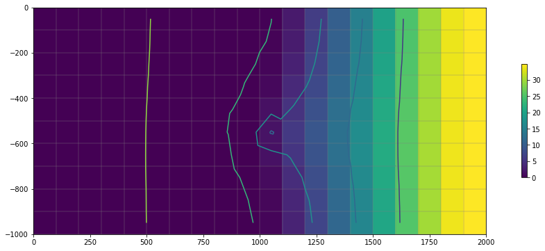
Datos de entrada
Puedes descargar los datos de entrada en este link.