Cálculo de esfuerzos efectivos desde un modelo hidrogeológico en MODFLOW con Flopy - Tutorial

La teoría de los esfuerzos efectivos fue desarrollada por Terzaghi en la década de 1920. Basándonos en nuestra experiencia en modelamiento queríamos calcular el esfuerzo efectivo en función de los resultados de un modelo de flujo de aguas subterráneas hecho en MODFLOW. Después de 6 años desde el primer planteamiento obtuvimos una deducción completa del cálculo del esfuerzo efectivo basado en la geometría y resultados del modelo y a la vez realizamos un ejemplo aplicado para el cálculo del esfuerzo efectivo en un modelo de flujo de agua subterránea de laderas/taludes.

El modelo de ejemplo se desarrolló en Modflow-Nwt y Model Muse, mientras que la determinación del esfuerzo efectivo se realizó con scripts en Python y Hataripy (nuestro “fork” de Flopy). Los scripts también pueden generar objetos 3D como archivos VTK de los resultados del modelo, la geometría y los esfuerzos efectivos que se pueden visualizar en Paraview.

Cálculo de tensión efectivo

Tutorial

Código

Este es el código en Python para el cálculo de los esfuerzos y la generación de geometrías.

import hataripy
import numpy as np
import matplotlib.pyplot as plt

hataripy is installed in C:\Users\saulm\anaconda3\lib\site-packages\hataripy

Open model and heads

#define model name, path, executables
modelWs = '../Model/'
modName = 'HillslopeModel_v1d_mf2005'
nwtPath = '../Exe/MODFLOW-NWT_64.exe'

#load model
mf = hataripy.modflow.Modflow.load(modName+'.nam', model_ws=modelWs, verbose=False,
                               check=False, exe_name=nwtPath)

# get a list of the model packages
mf.get_package_list()

['DIS', 'BAS6', 'OC', 'NWT', 'UPW', 'GHB', 'DRN', 'RCH']

# open binary head file
headFile = hataripy.utils.binaryfile.HeadFile(modelWs + modName + '.bhd')
headFile.get_times()

[1.0]

# get array of heads
headArray = headFile.get_data(totim=1.0)
headArray.shape

(20, 57, 46)

#plot surface topography
plt.imshow(mf.modelgrid.top)

<matplotlib.image.AxesImage at 0x28f1f09ac70>

Effective stress calculation

# calculate water table from heads
waterTableArray = np.zeros([headArray.shape[1],headArray.shape[2]])
for row in range(headArray.shape[1]):
    for col in range(headArray.shape[2]):
        heads=headArray[:,row,col]
        if heads[heads>-1e+20].size > 0:
            waterTableArray[row,col]=round(heads[heads>-1e+20][0],3)
        else:
            waterTableArray[row,col]=-1e+20

#plot water table
plt.imshow(waterTableArray)

<matplotlib.image.AxesImage at 0x28f1f819190>

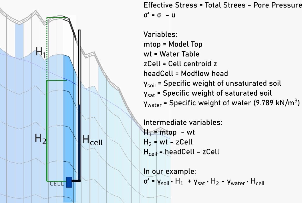
# H1 determination
H1 = np.zeros(headArray.shape)

for lay in range(headArray.shape[0]):
    H1[lay] = np.where((mf.modelgrid.top>waterTableArray)&(waterTableArray>mf.modelgrid.botm[lay]),
                       mf.modelgrid.top-waterTableArray,0)

# H2 determination
H2 = np.zeros(headArray.shape)

for lay in range(headArray.shape[0]):
    H2[lay] = np.where((mf.modelgrid.top>waterTableArray)&(waterTableArray>mf.modelgrid.zcellcenters[lay]),
                      waterTableArray-mf.modelgrid.zcellcenters[lay],0)

# HCell determination
HCell = np.zeros(headArray.shape)

for lay in range(headArray.shape[0]):
    oneCellHead = headArray[lay] - mf.modelgrid.zcellcenters[lay]
    HCell[lay] = np.where(oneCellHead>0, oneCellHead, 0)

rhoUnsat = 15 # in kN/m3 as reference value 
rhoSat = 19 # in kN/m3 as reference value 
rhoWater = 9.8 # in kN/m3

effectiveStress = rhoUnsat*H1 + rhoSat*H2 - rhoWater*HCell

#plot effective stresses for lay 1
plt.imshow(effectiveStress[0])

<matplotlib.image.AxesImage at 0x28f1f867ac0>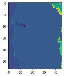

#plot effective stresses for row 25
plt.imshow(effectiveStress[:,25,:])

<matplotlib.image.AxesImage at 0x28f2088cf40>

Working on the VTK

# get information about the drain cells
drnCells = mf.drn.stress_period_data[0]

# get information about the ghb cells
ghbCells = mf.ghb.stress_period_data[0]

# add the arrays to the vtkObject
vtkObject = hataripy.export.vtk.Vtk3D(mf,'../vtuFiles/',verbose=True)
vtkObject.add_array('head',headArray)
vtkObject.add_array('drn',drnCells)
vtkObject.add_array('ghb',ghbCells)

# add the effective stress array
vtkObject.add_array('effectivestress',effectiveStress)

# Create the VTKs for model output, boundary conditions and water table
vtkObject.modelMesh('modelMesh.vtu',smooth=True,cellvalues=['head','effectivestress'])
vtkObject.modelMesh('modelDrn.vtu',smooth=True,cellvalues=['drn'],boundary='drn',avoidpoint=True)
vtkObject.modelMesh('modelGhb.vtu',smooth=True,cellvalues=['ghb'],boundary='ghb',avoidpoint=True)
vtkObject.waterTable('waterTable.vtu',smooth=True)

Writing vtk file: modelMesh.vtu
Number of point is 419520, Number of cells is 52440

Writing vtk file: modelDrn.vtu
Number of point is 2072, Number of cells is 259

Writing vtk file: modelGhb.vtu
Number of point is 11064, Number of cells is 1383

Writing vtk file: waterTable.vtu
Number of point is 10488, Number of cells is 2622