Conteo geoespacial de cultivos a partir de ortofotos de drones con Python, Scikit Learn y Scikit Image - Tutorial

Las ortofotos de drones nos proporcionan imágenes aéreas con resolución espacial en escala de centímetros. Con estas ortofotos de alta definición y bajo costo podemos interpretar, analizar y cuantificar objetos en una distribución horizontal mediante bibliotecas de “machine learning” para el reconocimiento de imágenes y análisis de conglomerados.

Hemos realizado un ejemplo aplicado de reconocimiento y conteo de plantas a partir de una ortofoto de drones con Python y las bibliotecas Scikit Learn y Scikit Image. Todo el proceso es geoespacial, ya que funciona con un ráster y un shapefile mostrando los resultados en QGIS.

Tutorial

Hay un tutorial anterior para disminuir la resolución de una ortofoto de drones en este enlace.

Datos de entrada

Puede descargar los datos de entrada desde este enlace.

Código

Este es el código completo del tutorial:

#import required libraries
%matplotlib inline
import matplotlib.pyplot as plt
import geopandas as gpd
import rasterio
from rasterio.plot import show
from skimage.feature import match_template
import numpy as np
from PIL import Image

C:\Users\GIDA2\Anaconda3\lib\site-packages\geopandas\_compat.py:88: UserWarning: The Shapely GEOS version (3.4.3-CAPI-1.8.3 r4285) is incompatible with the GEOS version PyGEOS was compiled with (3.8.1-CAPI-1.13.3). Conversions between both will be slow.
  shapely_geos_version, geos_capi_version_string

#open point shapefile
pointData = gpd.read_file('Shp/pointData.shp')
print('CRS of Point Data: ' + str(pointData.crs))

#open raster file
palmRaster = rasterio.open('Rst/palmaOrthoTotal_14cm.tif')
print('CRS of Raster Data: ' + str(palmRaster.crs))
print('Number of Raster Bands: ' + str(palmRaster.count))
print('Interpretation of Raster Bands: ' + str(palmRaster.colorinterp))

CRS of Point Data: epsg:4326
CRS of Raster Data: EPSG:4326
Number of Raster Bands: 4
Interpretation of Raster Bands: (<ColorInterp.red: 3>, <ColorInterp.green: 4>, <ColorInterp.blue: 5>, <ColorInterp.alpha: 6>)

#show point and raster on a matplotlib plot
fig, ax = plt.subplots(figsize=(18,18))
pointData.plot(ax=ax, color='orangered', markersize=100)
show(palmRaster, ax=ax)

C:\Users\GIDA2\Anaconda3\lib\site-packages\rasterio\plot.py:109: NodataShadowWarning: The dataset's nodata attribute is shadowing the alpha band. All masks will be determined by the nodata attribute
  arr = source.read(rgb_indexes, masked=True)





<matplotlib.axes._subplots.AxesSubplot at 0x1ccb236e6c8>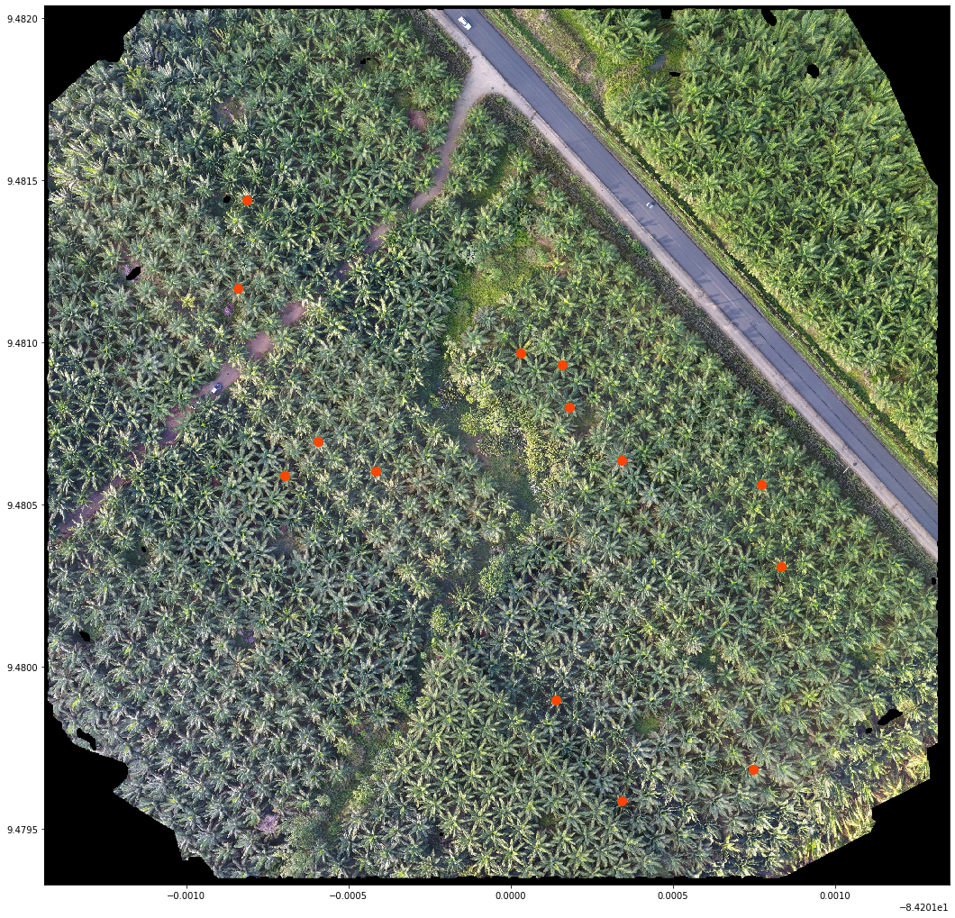

#selected band: green
greenBand = palmRaster.read(2)

#extract point value from raster
surveyRowCol = []
for index, values in pointData.iterrows():
    x = values['geometry'].xy[0][0]
    y = values['geometry'].xy[1][0]
    row, col = palmRaster.index(x,y)
    print("Point N°:%d corresponds to row, col: %d, %d"%(index,row,col))
    surveyRowCol.append([row,col])

Point N°:0 corresponds to row, col: 848, 1162
Point N°:1 corresponds to row, col: 875, 1263
Point N°:2 corresponds to row, col: 689, 471
Point N°:3 corresponds to row, col: 1693, 1246
Point N°:4 corresponds to row, col: 1940, 1408
Point N°:5 corresponds to row, col: 1864, 1727
Point N°:6 corresponds to row, col: 1368, 1796
Point N°:7 corresponds to row, col: 1168, 1748
Point N°:8 corresponds to row, col: 979, 1279
Point N°:9 corresponds to row, col: 1108, 1407
Point N°:10 corresponds to row, col: 1147, 586
Point N°:11 corresponds to row, col: 473, 494
Point N°:12 corresponds to row, col: 1062, 667
Point N°:13 corresponds to row, col: 1136, 808

# number of template images
print('Number of template images: %d'%len(surveyRowCol))
# define ratio of analysis
radio = 25

Number of template images: 14

#show all the points of interest, please be careful to have a complete image, otherwise the model wont run
fig, ax = plt.subplots(1, len(surveyRowCol),figsize=(20,5))

for index, item in enumerate(surveyRowCol):
    row = item[0]
    col = item[1]
    ax[index].imshow(greenBand)
    ax[index].plot(col,row,color='red', linestyle='dashed', marker='+',
     markerfacecolor='blue', markersize=8)
    ax[index].set_xlim(col-radio,col+radio)
    ax[index].set_ylim(row-radio,row+radio)
    ax[index].axis('off')
    ax[index].set_title(index)

# Match the image to the template

listaresultados = []

templateBandList = []
for rowCol in surveyRowCol:
    imageList = []
    row = rowCol[0]
    col = rowCol[1]
    #append original band
    imageList.append(greenBand[row-radio:row+radio, col-radio:col+radio])
    #append rotated images
    templateBandToRotate = greenBand[row-2*radio:row+2*radio, col-2*radio:col+2*radio]
    rotationList = [i*30 for i in range(1,4)]
    for rotation in rotationList:
        rotatedRaw = Image.fromarray(templateBandToRotate)
        rotatedImage = rotatedRaw.rotate(rotation)
        imageList.append(np.asarray(rotatedImage)[radio:-radio,radio:-radio])
    #plot original and rotated images
    fig, ax = plt.subplots(1, len(imageList),figsize=(12,12))
    for index, item in enumerate(imageList):
        ax[index].imshow(imageList[index])
    #add images to total list
    templateBandList+=imageList

# match the template image to the orthophoto
matchXYList = []
for index, templateband in enumerate(templateBandList):
    if index%10 == 0:
        print('Match template ongoing for figure Nº %d'%index)
    matchTemplate = match_template(greenBand, templateband, pad_input=True)
    matchTemplateFiltered = np.where(matchTemplate>np.quantile(matchTemplate,0.9996))
    for item in zip(matchTemplateFiltered[0],matchTemplateFiltered[1]):
        x, y = palmRaster.xy(item[0], item[1])
        matchXYList.append([x,y])

Match template ongoing for figure Nº 0
Match template ongoing for figure Nº 10
Match template ongoing for figure Nº 20
Match template ongoing for figure Nº 30
Match template ongoing for figure Nº 40
Match template ongoing for figure Nº 50

# plot interpreted points over the image
fig, ax = plt.subplots(figsize=(20, 20))
matchXYArray = np.array(matchXYList)
ax.scatter(matchXYArray[:,0],matchXYArray[:,1], marker='o',c='orangered', s=100, alpha=0.25)
show(palmRaster, ax=ax)

<matplotlib.axes._subplots.AxesSubplot at 0x1ccba1d7408>

# cluster analysis
from sklearn.cluster import Birch
brc = Birch(branching_factor=10000, n_clusters=None, threshold=2e-5, compute_labels=True)
brc.fit(matchXYArray)
birchPoint = brc.subcluster_centers_
birchPoint

array([[-84.20038278,   9.48201204],
       [-84.20064248,   9.48201099],
       [-84.20022459,   9.48195993],
       ...,
       [-84.20154469,   9.4803915 ],
       [-84.20115389,   9.47998263],
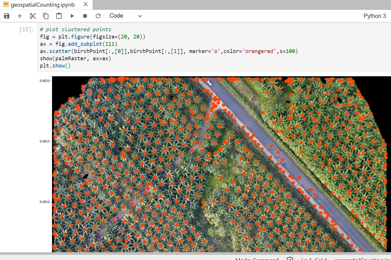
       [-84.20024387,   9.47971317]])

# plot clustered points
fig = plt.figure(figsize=(20, 20))
ax = fig.add_subplot(111)
ax.scatter(birchPoint[:,[0]],birchPoint[:,[1]], marker='o',color='orangered',s=100)
show(palmRaster, ax=ax)
plt.show()

# save xy to a csv file
np.savetxt("Txt/birchPoints.csv", birchPoint, delimiter=",")