Determinación de un Cono de Depresión de un Tajo Abierto con Python, Flopy y mfVoronoi - Tutorial

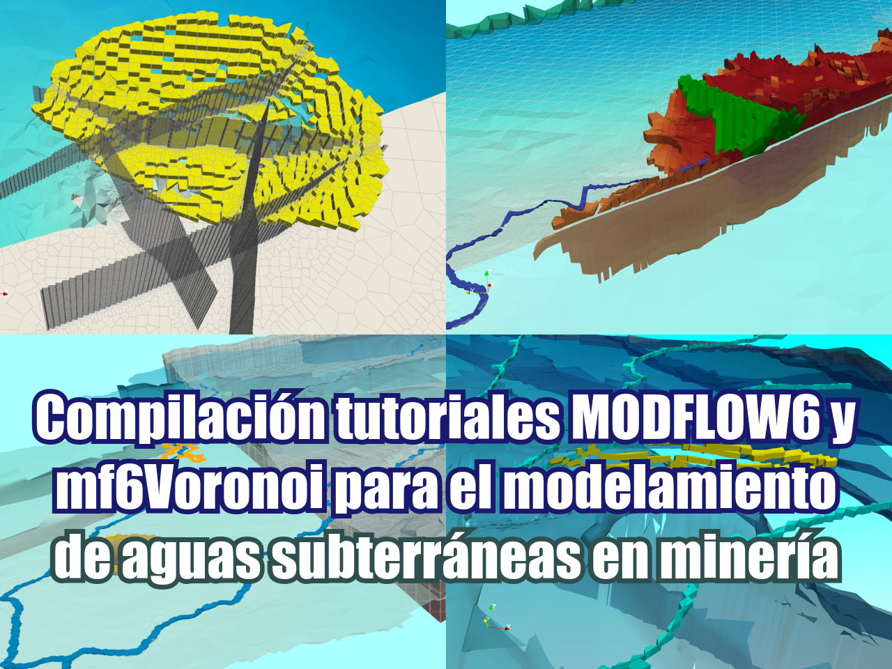
Uno de los objetivos clave de la modelación de aguas subterráneas en minería es la determinación de los ingresos de agua al tajo y la extensión del cono de depresión. Este tutorial muestra un caso aplicado de determinación de un cono de depresión a partir de un modelo de tajo abierto construido con MODFLOW6, Flopy y mf6Voronoi. El modelo incluye fallas geológicas y el tutorial cubre todos los pasos, desde la importación del modelo, el procesamiento de datos y la exportación de datos geoespaciales del cono de depresión.

Este tutorial esta basado en los datos de este otro tutorial:

gidahatari.com/ih-es/implementacin-de-fallas-y-zone-budgets-en-un-modelo-modflow6-voronoi-para-tajo-abierto-tutorial

Tutorial

Código

#Vtk generation
import flopy ## Org
import rasterio 
from rasterio.plot import show
from mf6Voronoi.tools.graphs2d import generateRasterFromArray, generateContoursFromRaster

C:\Users\saulm\anaconda3\Lib\site-packages\geopandas\_compat.py:7: DeprecationWarning: The 'shapely.geos' module is deprecated, and will be removed in a future version. All attributes of 'shapely.geos' are available directly from the top-level 'shapely' namespace (since shapely 2.0.0).
  import shapely.geos

# load simulation
simName = 'mf6Sim' ## Org
modelName = 'mf6Model' ## Org
modelWs = 'modelFiles' ## Org
sim = flopy.mf6.MFSimulation.load(sim_name=modelName, version='mf6', ## Org
                             exe_name='bin/mf6.exe', ## Org
                             sim_ws=modelWs) ## Org

loading simulation...
  loading simulation name file...
  loading tdis package...
  loading model gwf6...
    loading package disv...
    loading package ic...
    loading package npf...
    loading package sto...
    loading package rch...
    loading package evt...
    loading package drn...
    loading package oc...
  loading solution package mf6model...

#list model
sim.model_names

['mf6model']

#get gwf
gwf = sim.get_model('mf6model')

headObj = gwf.output.head() ## Org
headObj.get_kstpkper() ## Org

[(0, 0), (0, 1), (0, 2), (0, 3), (0, 4), (0, 5)]

heads0 = headObj.get_data(kstpkper=(0,0)) ## Org
heads5 = headObj.get_data(kstpkper=(0,5)) ## Org

waterTable0 = flopy.utils.postprocessing.get_water_table(heads0) ## Org
waterTable5 = flopy.utils.postprocessing.get_water_table(heads5) ## Org

wt0Path = 'output/waterTable0.tif'
wt5Path = 'output/waterTable5.tif'

generateRasterFromArray(gwf, waterTable0, 
                        rasterRes=10, epsg=32612, 
                        outputPath=wt0Path,
                        limitLayer='shp/catchment.shp')
generateRasterFromArray(gwf, waterTable5, 
                        rasterRes=10, epsg=32612, 
                        outputPath=wt5Path,
                        limitLayer='shp/catchment.shp')

Raster X Dim: 13256.95, Raster Y Dim: 9903.42
Number of cols:  1325, Number of rows: 990
Raster X Dim: 13256.95, Raster Y Dim: 9903.42
Number of cols:  1325, Number of rows: 990

wt0 = rasterio.open(wt0Path)
show(wt0)

wt0Clip = rasterio.open('output/waterTable0_clip.tif')
show(wt0Clip)

depressionArray = waterTable5 - waterTable0
depressionPath = 'output/depression.tif'
generateRasterFromArray(gwf, depressionArray, 
                        rasterRes=10, epsg=32612, 
                        outputPath=depressionPath,
                        limitLayer='shp/catchment.shp')

Raster X Dim: 13256.95, Raster Y Dim: 9903.42
Number of cols:  1325, Number of rows: 990

generateContoursFromRaster('output/depression.tif',5,
                           'output/depressionContours.shp')

Datos de entrada

owncloud.hatarilabs.com/s/dYnmmUm3byXxMe4

Password: Hatarilabs