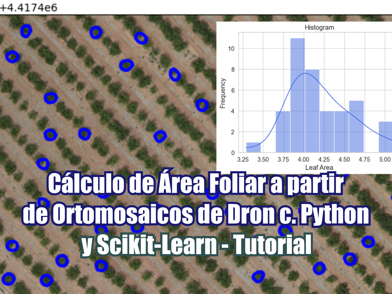
Además de contar cultivos, también podemos delinear plantas y calcular su área foliar utilizando métodos que ajustan splines abiertos o cerrados a líneas o bordes en una imagen. Estos métodos están implementados en la biblioteca de Python Scikit-Image y se aplican para la delineación de copas de árboles sobre una imagen ráster geoespacial. El ejercicio se desarrolla en un Jupyter Notebook y cubre todos los pasos: desde la importación de la imagen, aplicación de escala de grises, exploración del filtro gaussiano, cálculo de contornos activos y exportación de polígonos como shapefile de ESRI. Finalmente, se genera un histograma para determinar la distribución del área foliar de las plantas.
Tutorial
Parte 1
Parte 2
Codigo
#open the required packages
import numpy as np
import seaborn as sns
import matplotlib.pyplot as plt

import rasterio
from rasterio.plot import show
import geopandas as gpd
from shapely.geometry import Polygon

from skimage.color import rgb2gray
from skimage import data
from skimage.filters import gaussian
from skimage.segmentation import active_contour, chan_vese
#open the raster file with rasterio
imgObj = rasterio.open('../orthophotos/olivosBorrianaClipCoarse.tif')
imgBand = imgObj.read(1)#explore the raster units and resolution
units = imgObj.crs.linear_units
res = imgObj.res
print("Raster unit is %s and resolution is %.2f"%(units,res[0]))Raster unit is metre and resolution is 0.02#aprox cell diameter = 2.5m, get cell radius in meters
cellRad = int(2.5/2//imgObj.res[0])
print(cellRad)50#working with a greyscaled version of the image
hatariIndex = 0.2125 * imgObj.read(1) + 0.7154 * imgObj.read(2) \
+ 0.0721 * imgObj.read(3)
plt.imshow(hatariIndex)
plt.show()
#olive points
olivPoints = gpd.read_file('../outShp/birchCrop2.shp')

#for one olive
olPt = olivPoints.iloc[0].geometry
x,y = olPt.x, olPt.y
print(x)745709.4467275749#explore the gaussian filter
gaussImg = gaussian(hatariIndex, sigma=2, preserve_range=False)
plt.imshow(gaussImg)<matplotlib.image.AxesImage at 0x1af8fd2c620>
#create a circle around the tree
row,col = imgObj.index(x,y)

s = np.linspace(0, 2 * np.pi, 20)
r = row + cellRad * np.sin(s)
c = col + cellRad * np.cos(s)
init = np.array([r, c]).T

init[:5]
array([[2110. , 3466. ],
[2126.23497346, 3463.29086209],
[2140.71063563, 3455.45702547],
[2151.85832391, 3443.34740791],
[2158.4700133 , 3428.27427436]])snake = active_contour(
gaussImg,
init,
alpha=0.015,
# beta=1.0,
# gamma=0.25,
#w_line=-15,
#w_edge=15,
max_num_iter=150,
boundary_condition='periodic'
)fig, ax = plt.subplots(figsize=(7, 7))
ax.imshow(hatariIndex, cmap=plt.cm.gray)
ax.plot(init[:, 1], init[:, 0], '--r', lw=3)
ax.plot(snake[:, 1], snake[:, 0], '-b', lw=3)
ax.set_xlim(col-800,col+800)
ax.set_ylim(row-800,row+800)
ax.invert_yaxis()
plt.show()
def rowColToXy(snake):
    xyList = []
    for vertex in snake:
        x,y = imgObj.xy(vertex[0],vertex[1])
        xyList.append([x,y])
    return xyList
sampleList = rowColToXy(snake)
sampleList[:5][[745710.7453, 4417425.881924019],
[745710.6775715511, 4417425.466312238],
[745710.4817256352, 4417425.070553344],
[745710.1789851976, 4417424.7918397],
[745709.8021568588, 4417424.5765464995]]snakeXyList = []
initList = []
for index, row in olivPoints.iloc[:40].iterrows():
olPt = olivPoints.iloc[index].geometry
x,y = olPt.x, olPt.y
#create a circle around the tree
row,col = imgObj.index(x,y)
s = np.linspace(0, 2 * np.pi, 20)
r = row + cellRad * np.sin(s)
c = col + cellRad * np.cos(s)
print("Working for index %d"%index)
init = np.array([r, c]).T
initList.append(init)
snake = active_contour(
gaussian(hatariIndex, sigma=3, preserve_range=False),
init,
alpha=0.015,
max_num_iter=150,
boundary_condition='periodic'
)
snakeXyList.append(rowColToXy(snake))Working for index 0
Working for index 1
Working for index 2
Working for index 3
Working for index 4
Working for index 5
Working for index 6
Working for index 7
Working for index 8
Working for index 9
Working for index 10
Working for index 11
Working for index 12
Working for index 13
Working for index 14
Working for index 15
Working for index 16
Working for index 17
Working for index 18
Working for index 19
Working for index 20
Working for index 21
Working for index 22
Working for index 23
Working for index 24
Working for index 25
Working for index 26
Working for index 27
Working for index 28
Working for index 29
Working for index 30
Working for index 31
Working for index 32
Working for index 33
Working for index 34
Working for index 35
Working for index 36
Working for index 37
Working for index 38
Working for index 39fig, ax = plt.subplots(figsize=(7, 7))
show(imgObj, ax=ax)
for snake in snakeXyList:
snake = np.array(snake)
ax.plot(snake[:, 0], snake[:, 1], '-b', lw=3)
plt.show()
polygons = [Polygon(coords) for coords in snakeXyList]
gdf = gpd.GeoDataFrame(geometry=polygons)
gdf.set_crs(olivPoints.crs, inplace=True)
gdf.to_file("../outShp/leafArea.shp", driver="ESRI Shapefile")
polyDf = gpd.read_file("../outShp/leafArea.shp")
polyDf.plot()<Axes: >
polyDf['area'] = polyDf.geometry.area

sns.set(style="whitegrid", palette="muted", font_scale=1.2)

# Create histogram
sns.histplot(polyDf['area'], bins=10, kde=True, color="royalblue",
                edgecolor="white")

# Customize plot
plt.title("Histogram")
plt.xlabel("Leaf Area")
plt.ylabel("Frequency")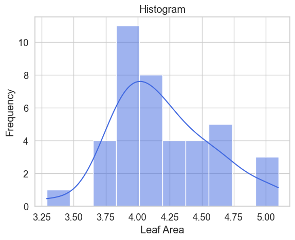
Datos de ingreso
Puede descargar los datos de ingreso desde este enlace:
owncloud.hatarilabs.com/s/0lccEhvuEfoiG7c
Password para descargar datos: Hatarilabs