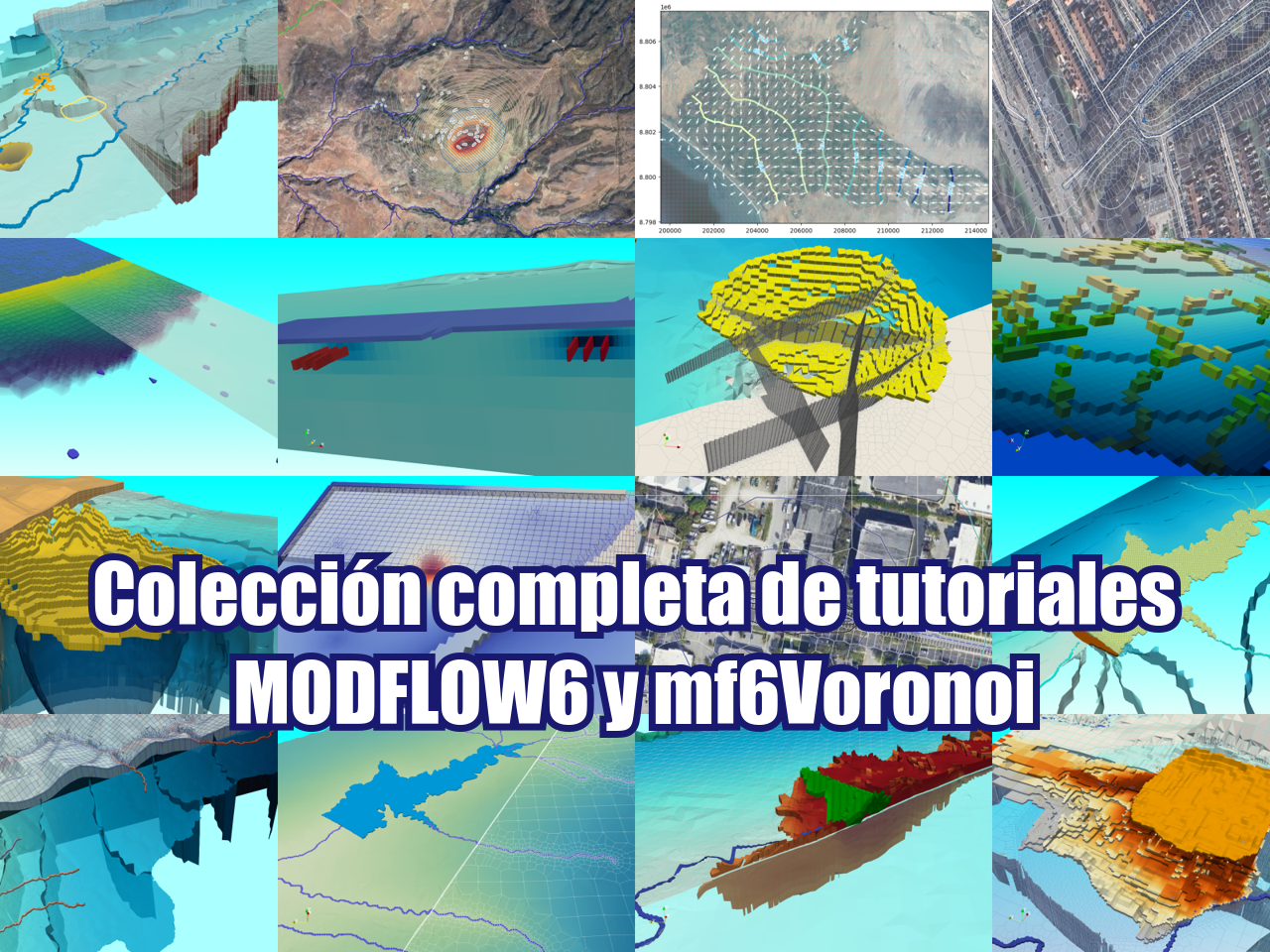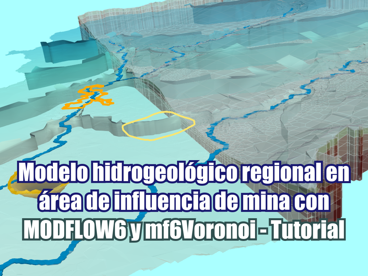
A veces se requieren modelos regionales como insumo para modelos locales de flujo y transporte. Este es un caso aplicado de modelación de aguas subterráneas a escala regional en el estado de Guerrero, México, que servirá como insumo para futuros modelos locales de abatimiento en tajos y transporte de contaminantes desde la presa de relaves y el depósito de desmonte. El modelo de aguas subterráneas está construido con MODFLOW6 y mf6Voronoi en una serie de Jupyter Notebooks, y los resultados se visualizan con Paraview.
Tutorial
Datos de ingreso
owncloud.hatarilabs.com/s/81eniQRXkWik142
Password para descargar: Hatarilabs
Código
Este es el código para la segunda parte del tutorial relacionado con la construcción y simulación del modelo de aguas subterráneas.
Part 2a: generate disv properties
import sys, json, os ## Org
import rasterio, flopy ## Org
import numpy as np ## Org
import matplotlib.pyplot as plt ## Org
import geopandas as gpd ## Org
from mf6Voronoi.meshProperties import meshShape ## Org
from shapely.geometry import MultiLineString ## Org
C:\Users\saulm\anaconda3\Lib\site-packages\geopandas\_compat.py:7: DeprecationWarning: The 'shapely.geos' module is deprecated, and will be removed in a future version. All attributes of 'shapely.geos' are available directly from the top-level 'shapely' namespace (since shapely 2.0.0).
import shapely.geos# open the json file
with open('../json/disvDict.json') as file: ## Org
gridProps = json.load(file) ## Orgcell2d = gridProps['cell2d'] #cellid, cell centroid xy, vertex number and vertex id list
vertices = gridProps['vertices'] #vertex id and xy coordinates
ncpl = gridProps['ncpl'] #number of cells per layer
nvert = gridProps['nvert'] #number of verts
centroids=gridProps['centroids'] #cell centroids xyPart 2b: Model construction and simulation
#Extract dem values for each centroid of the voronois
src = rasterio.open('../rst/clipDem100m.tif')  ## Org
elevation=[x for x in src.sample(centroids)] ## Org
nlay = 5 ## Org
mtop=np.array([elev[0] for i,elev in enumerate(elevation)]) ## Org
zbot=np.zeros((nlay,ncpl)) ## Org
AcuifInf_Bottom = 100 ## Org
zbot[0,] = mtop - 20 ## Org
zbot[1,] = AcuifInf_Bottom + (0.85 * (mtop - AcuifInf_Bottom)) ## Org
zbot[2,] = AcuifInf_Bottom + (0.70 * (mtop - AcuifInf_Bottom)) ## Org
zbot[3,] = AcuifInf_Bottom + (0.50 * (mtop - AcuifInf_Bottom)) ## Org
zbot[4,] = AcuifInf_Bottom ## OrgCreate simulation and model
# create simulation
simName = 'mf6Sim' ## Org
modelName = 'mf6Model' ## Org
modelWs = '../modelFiles' ## Org
sim = flopy.mf6.MFSimulation(sim_name=modelName, version='mf6', ## Org
                             exe_name='../bin/mf6.exe', ## Org
                             sim_ws=modelWs) ## Org
# create tdis package
tdis_rc = [(1000.0, 1, 1.0)] ## Org
tdis = flopy.mf6.ModflowTdis(sim, pname='tdis', time_units='SECONDS', ## Org
perioddata=tdis_rc) ## Org# create gwf model
gwf = flopy.mf6.ModflowGwf(sim, ## Org
modelname=modelName, ## Org
save_flows=True, ## Org
newtonoptions="NEWTON UNDER_RELAXATION") ## Org# create iterative model solution and register the gwf model with it
ims = flopy.mf6.ModflowIms(sim, ## Org
complexity='COMPLEX', ## Org
outer_maximum=50, ## Org
inner_maximum=30, ## Org
linear_acceleration='BICGSTAB') ## Org
sim.register_ims_package(ims,[modelName]) ## Org# disv
disv = flopy.mf6.ModflowGwfdisv(gwf, nlay=nlay, ncpl=ncpl, ## Org
top=mtop, botm=zbot, ## Org
nvert=nvert, vertices=vertices, ## Org
cell2d=cell2d) ## Org# initial conditions
ic = flopy.mf6.ModflowGwfic(gwf, strt=np.stack([mtop for i in range(nlay)])) ## OrgKx =[4E-4,5E-6,1E-6,9E-7,5E-7] ## Org
icelltype = [1,1,0,0,0] ## Org
# node property flow
npf = flopy.mf6.ModflowGwfnpf(gwf, ## Org
save_specific_discharge=True, ## Org
icelltype=icelltype, ## Org
k=Kx) ## Org## <==== inserted
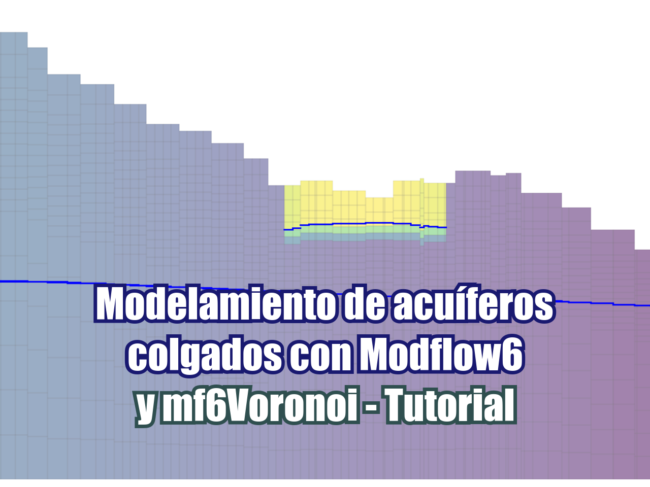
crossSection = gpd.read_file('../shp/crossSection.shp') ## <==== inserted
sectionLine =list(crossSection.iloc[0].geometry.coords) ## <==== inserted
fig, ax = plt.subplots(figsize=(12,8)) ## <==== inserted
modelxsect = flopy.plot.PlotCrossSection(model=gwf, line={'Line': sectionLine}) ## <==== inserted
linecollection = modelxsect.plot_grid(lw=0.5) ## <==== inserted
modelxsect.plot_array(np.log(npf.k.array), alpha=0.5) ## <====== inserted
ax.grid() ## <==== inserted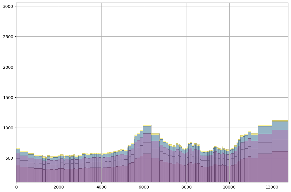
# define storage and transient stress periods
sto = flopy.mf6.ModflowGwfsto(gwf, ## Org
                              iconvert=1, ## Org
                              steady_state={ ## Org
                                0:True, ## Org
                              } ## Org
                              ) ## Org
Working with rechage, evapotranspiration
rchr = 0.15/365/86400 ## Org
rch = flopy.mf6.ModflowGwfrcha(gwf, recharge=rchr) ## Org
evtr = 1.2/365/86400 ## Org
evt = flopy.mf6.ModflowGwfevta(gwf,ievt=1,surface=mtop,rate=evtr,depth=1.0) ## Org
Definition of the intersect object
For the manipulation of spatial data to determine hydraulic parameters or boundary conditions
# Define intersection object
interIx = flopy.utils.gridintersect.GridIntersect(gwf.modelgrid) ## Org#open the river shapefile
rivers =gpd.read_file('../hatariUtils/river_basin.shp') ## Org
list_rivers=[] ## Org
for i in range(rivers.shape[0]): ## Org
list_rivers.append(rivers['geometry'].loc[i]) ## Org
riverMls = MultiLineString(lines=list_rivers) ## Org
#intersec rivers with our grid
riverCells=interIx.intersect(riverMls).cellids ## Org
riverCells[:10] ## Orgarray([252, 275, 291, 321, 336, 344, 370, 434, 441, 446], dtype=object)#river package
riverSpd = {} ## Org
riverSpd[0] = [] ## Org
for cell in riverCells: ## Org
riverSpd[0].append([(0,cell),mtop[cell],0.01]) ## Org
riv = flopy.mf6.ModflowGwfdrn(gwf, stress_period_data=riverSpd) ## Org#river plot
riv.plot(mflay=0) ## Org[<Axes: title={'center': ' drn_0 location stress period 1 layer 1'}>]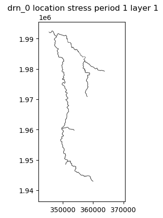
Set the Output Control and run simulation
#oc
head_filerecord = f"{gwf.name}.hds" ## Org
budget_filerecord = f"{gwf.name}.cbc" ## Org
oc = flopy.mf6.ModflowGwfoc(gwf, ## Org
                            head_filerecord=head_filerecord, ## Org
                            budget_filerecord = budget_filerecord, ## Org
                            saverecord=[("HEAD", "LAST"),("BUDGET","LAST")]) ## Org
# Run the simulation
sim.write_simulation() ## Org
success, buff = sim.run_simulation() ## Orgwriting simulation...
writing simulation name file...
writing simulation tdis package...
writing solution package ims_-1...
writing model mf6Model...
writing model name file...
writing package disv...
writing package ic...
writing package npf...
writing package sto...
writing package rcha_0...
writing package evta_0...
writing package drn_0...
INFORMATION: maxbound in ('gwf6', 'drn', 'dimensions') changed to 929 based on size of stress_period_data
writing package oc...
FloPy is using the following executable to run the model: ..\bin\mf6.exe
MODFLOW 6
U.S. GEOLOGICAL SURVEY MODULAR HYDROLOGIC MODEL
VERSION 6.6.0 12/20/2024
MODFLOW 6 compiled Dec 31 2024 17:10:16 with Intel(R) Fortran Intel(R) 64
Compiler Classic for applications running on Intel(R) 64, Version 2021.7.0
Build 20220726_000000
This software has been approved for release by the U.S. Geological
Survey (USGS). Although the software has been subjected to rigorous
review, the USGS reserves the right to update the software as needed
pursuant to further analysis and review. No warranty, expressed or
implied, is made by the USGS or the U.S. Government as to the
functionality of the software and related material nor shall the
fact of release constitute any such warranty. Furthermore, the
software is released on condition that neither the USGS nor the U.S.
Government shall be held liable for any damages resulting from its
authorized or unauthorized use. Also refer to the USGS Water
Resources Software User Rights Notice for complete use, copyright,
and distribution information.
MODFLOW runs in SEQUENTIAL mode
Run start date and time (yyyy/mm/dd hh:mm:ss): 2025/07/11 16:14:46
Writing simulation list file: mfsim.lst
Using Simulation name file: mfsim.nam
Solving: Stress period: 1 Time step: 1
Run end date and time (yyyy/mm/dd hh:mm:ss): 2025/07/11 16:14:53
Elapsed run time: 6.815 Seconds
Normal termination of simulation.Model output visualization
headObj = gwf.output.head() ## Org
headObj.get_kstpkper() ## Org
[(0, 0)]heads = headObj.get_data() ## Org
heads[2,0,:5] ## Orgarray([1016.74658849, 1003.30308189, 1016.19148927, 1015.36206045,
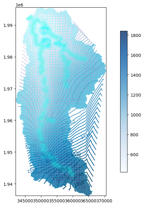
1017.46065387])# Plot the heads for a defined layer and boundary conditions
fig = plt.figure(figsize=(12,8)) ## Org
ax = fig.add_subplot(1, 1, 1, aspect='equal') ## Org
modelmap = flopy.plot.PlotMapView(model=gwf) ## Org
####
levels = np.linspace(heads[heads>-1e+30].min(),heads[heads>-1e+30].max(),num=50) ## Org
contour = modelmap.contour_array(heads[3],ax=ax,levels=levels,cmap='PuBu') ## Org
ax.clabel(contour) ## Org
quadmesh = modelmap.plot_bc('DRN') ## Org
cellhead = modelmap.plot_array(heads[3],ax=ax, cmap='Blues', alpha=0.8) ## Org
linecollection = modelmap.plot_grid(linewidth=0.3, alpha=0.5, color='cyan', ax=ax) ## Org
plt.colorbar(cellhead, shrink=0.75) ## Org
plt.show() ## Org