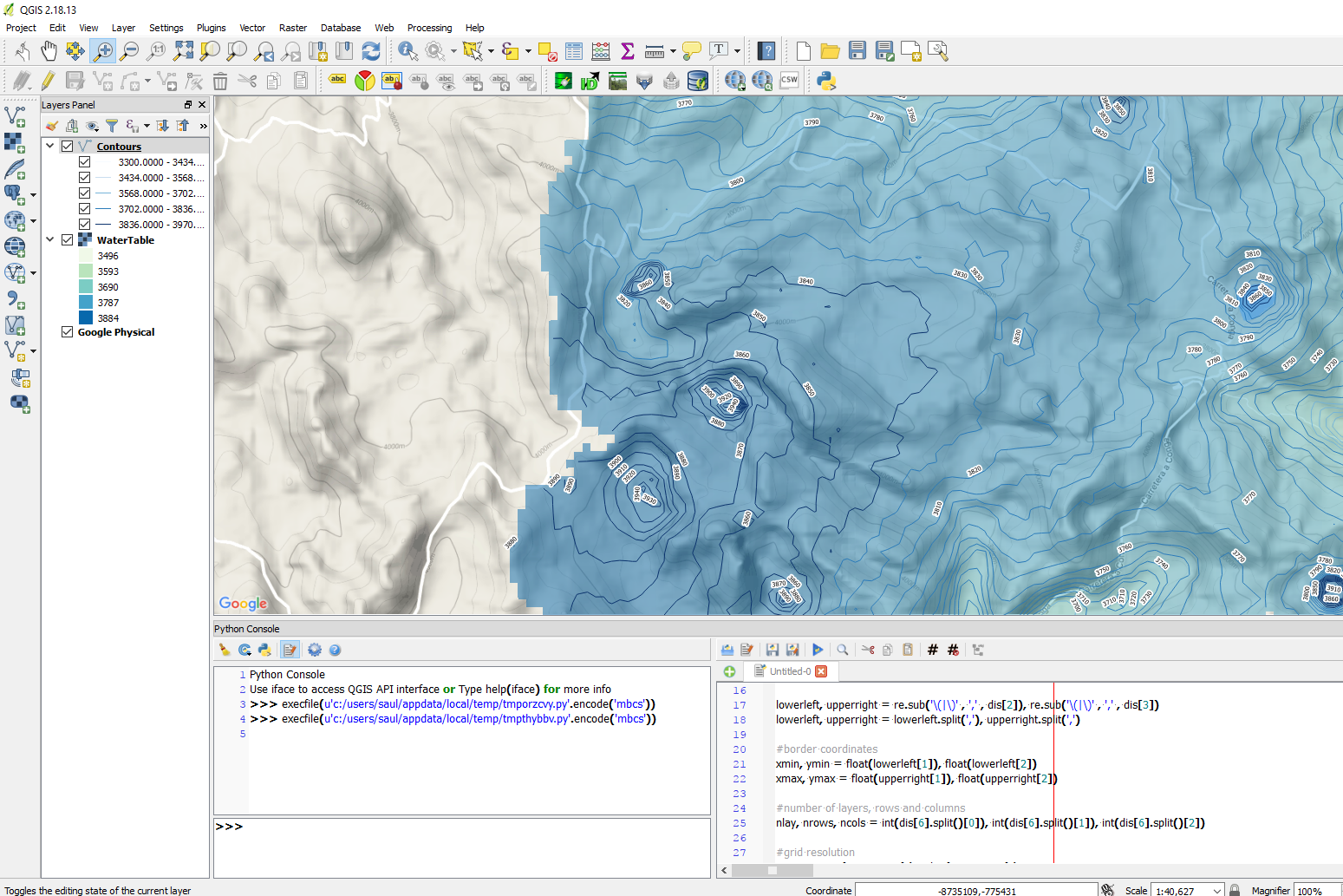
Tutorial para Representar la Napa Freática de MODFLOW en QGIS con Python

Las capacidades actuales de modelamiento de acuíferos con MODFLOW y Model Muse nos permiten grandes refinamientos y mayor número de capas para la representación de las cargas hidráulicas y la napa freática así como mayores capacidades para la representación de los procesos físicos relacionados al flujo de aguas subterráneas. En una escala regional podemos estar tratando con modelos de mas de 50000 elementos en régimen uniforme o transitorio, de los cuales muchas veces necesitamos representar sus datos en plataformas de Sistemas de Información Geográfica (SIG) como QGIS para un mayor análisis o la generación de gráficos para usuarios finales y actores de decisión. El uso de programación en Python nos permite acelerar el proceso de la representación de datos de salida de MODFLOW en QGIS.

Los scripts en Python pueden ser un poco largos y declarativos, pero el tiempo de procesamiento es mucho menor comparado con el uso de la interface visual. Se pretende que los modeladores guarden estos scripts y los usen cada vez quieran representar los datos de la napa freática.

Tutorial

Código

Este es el código completo en Python desde la consola de QGIS:

#####
#Part1
#####

#import the required libraries
import matplotlib.pyplot as plt
import os, re
import numpy as np
from osgeo import gdal, gdal_array, osr

#change directory to the model files path
os.chdir('C:\Users\Saul\Documents\Ih_MODFLOWResultsinQGIS\Model')

#open the *.DIS file and get the model boundaries and discretization
dis= open('Modelo1.dis').readlines()

lowerleft, upperright = re.sub('\(|\)' , ',' , dis[2]), re.sub('\(|\)' , ',' , dis[3])
lowerleft, upperright = lowerleft.split(','), upperright.split(',')

#border coordinates
xmin, ymin = float(lowerleft[1]), float(lowerleft[2])
xmax, ymax = float(upperright[1]), float(upperright[2])

#number of layers, rows and columns
nlay, nrows, ncols = int(dis[6].split()[0]), int(dis[6].split()[1]), int(dis[6].split()[2])

#grid resolution
xres, yres = (xmax-xmin)/ncols, (ymax-ymin)/nrows



#####
#Part2
#####

#open the *.FHD file to read the heads, beware that the script runs only on static models
hds = open('Modelo1.fhd').readlines()

#lines that separate heads from a layer
breakers=[x for x in range(len(hds)) if hds[x][:4]=='    ']

#counter plus a empty numpy array for model results
i=0
headmatrix = np.zeros((nlay,nrows,ncols))

#loop to read all the heads in one layer, reshape them to the grid dimensions and add to the numpy array
for salto in breakers:
    rowinicio = salto + 1
    rowfinal = salto + 2545 #here we insert the len of lines per layer
    matrixlist = []
    
    for linea in range(rowinicio,rowfinal,1):
        listaitem = [float(item) for item in hds[linea].split()]
        for item in listaitem: matrixlist.append(item)
 
    matrixarray = np.asarray(matrixlist)
    matrixarray = matrixarray.reshape(nrows,ncols)
    
    headmatrix[i,:,:]=matrixarray
    i+=1

#empty numpy array for the water table
wt = np.zeros((nrows,ncols))

#obtain the first positive or real head from the head array
for row in range(nrows):
    for col in range(ncols):
        a = headmatrix[:,row,col]
        if a[a>-1000] != []:                    #just in case there are some inactive zones
            wt[row,col] = a[a>-1000][0]
        else: wt[row,col] = None



#####
#Part3
#####

#definition of the raster name
outputraster = "waterlevel.tif"

#delete output raster if exits
try:
    os.remove(outputraster)
except OSError:
    pass

#creation of a raster and parameters for the array geotransformation
geotransform = [xmin,xres,0,ymax,0,-yres]
raster = gdal.GetDriverByName('GTiff').Create(outputraster,ncols,nrows,1,gdal.GDT_Float32)
raster.SetGeoTransform(geotransform)

#assign of a spatial reference by EPSG code
srs=osr.SpatialReference()
srs.ImportFromEPSG(32717)

#write results on the created raster
raster.SetProjection(srs.ExportToWkt())
raster.GetRasterBand(1).WriteArray(wt)

#add the raster to the canvas
iface.addRasterLayer(outputraster,"WaterTable","gdal")