Modelamiento de la especiación del agua de mar con Phreeqc acoplado a Python y Pandas - Tutorial

El modelo de especiación permite calcular la distribución de especies acuosas en una solución. Phreeqc es capaz de simular este cálculo de especiación y vamos a demostrar esta capacidad en un caso de estudio de especies acuosas en agua de mar.

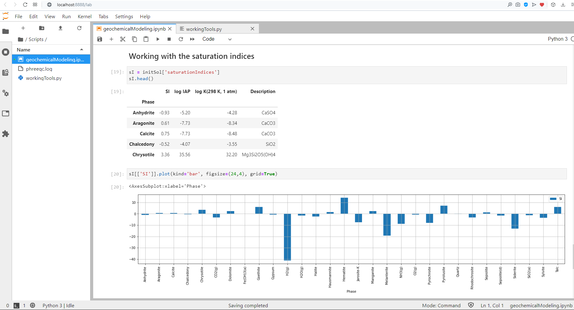
Hemos realizado un tutorial para el modelamiento de especiación de agua de mar con Phreeqc que se ejecuta en Python en un entorno de Jupyter Lab. El código puede correr el ejecutable Phreeqc, definir las bases de datos y establecer los archivos de salida. Los resultados de la simulación están disponibles como dataframes de Pandas y se realizan gráficos para los componentes principales y la distribución de los índices de saturación.

Tutorial

Código

# This tutorial works on Windows and might work on Linux althought it have not been tested. 
# You need to have the batch version of Phreeqc installed
# Download Phreeqc from: https://www.usgs.gov/software/phreeqc-version-3

# import required packages and classes
import os
from workingTools import phreeqcModel
from pathlib import Path

Create a Phreeqc object, define executables and databases

#define the model object
chemModel = phreeqcModel()

#assing the executable and database
phPath = "C:\\Program Files\\USGS\\phreeqc-3.6.2-15100-x64"
chemModel.phBin = os.path.join(phPath,"bin\\phreeqc.bat")
chemModel.phDb = os.path.join(phPath,"database\\phreeqc.dat")
chemModel.phDb

'C:\\Program Files\\USGS\\phreeqc-3.6.2-15100-x64\\database\\phreeqc.dat'

Set the input and output files

chemModel.inputFile = Path("../In/ex1a.in")
chemModel.outputFile = Path("../Out/ex1.out")
chemModel.inputFile

WindowsPath('../In/ex1a.in')

Run model and show simulation data

chemModel.runModel()

Input file: ..\In\ex1a.in

Output file: ..\Out\ex1.out

Database file: C:\Program Files\USGS\phreeqc-3.6.2-15100-x64\database\phreeqc.dat



                           * PHREEQC-3.6.2 *              

                    A hydrogeochemical transport model    

                                  by                      
                     D.L. Parkhurst and C.A.J. Appelo     

                            January 28, 2020              



Simulation 1. Initial solution 1.        /                                             

End of Run after 1.666 Seconds.

chemModel.showSimulations()

Parsing output file: 1 simulations found
Simulation 1:  Example 1a.--Speciate seawater. from line 18 to 261

Show simulation components

simObj = chemModel.getSimulation(1)

Simulation content:
        Initial solution calculation: True
        Batch reaction calculations: False
        Number of reactions steps: 0

# In case you need more information about the line interval of the output file
#simObj.getSimulationDict()

Get initial solution

initSol = simObj.getInitialSolution()
initSol.keys()

dict_keys(['solutionComposition', 'descriptionSolution', 'redoxCouples', 'distributionSpecies', 'saturationIndices'])

iS = initSol['solutionComposition']
iS

	Molality	Moles	Description
Elements
Alkalinity	2.406000e-03	2.406000e-03	None
Ca	1.066000e-02	1.066000e-02	None
Cl	5.657000e-01	5.657000e-01	None
Fe	3.711000e-08	3.711000e-08	None
K	1.058000e-02	1.058000e-02	None
Mg	5.507000e-02	5.507000e-02	None
Mn	3.773000e-09	3.773000e-09	None
N(-3)	1.724000e-06	1.724000e-06	None
N(5)	4.847000e-06	4.847000e-06	None
Na	4.854000e-01	4.854000e-01	None
O(0)	4.376000e-04	4.376000e-04	Equilibrium with O2(g)
S(6)	2.926000e-02	2.926000e-02	None
Si	7.382000e-05	7.382000e-05	None

iS[['Molality']].plot(kind='bar', grid=True)

<AxesSubplot:xlabel='Elements'>

dS = initSol['descriptionSolution']
dS

	Value
Parameter
pH	8.220000
pe	8.451000
Specific Conductance (µS/cm, [0-9]5°C)	52630.000000
Density (g/cm³)	1.023230
Volume (L)	1.012820
Activity of water	0.981000
Ionic strength (mol/kgw)	0.674700
Mass of water (kg)	1.000000
Total carbon (mol/kg)	0.002182
Total CO2 (mol/kg)	0.002182
Temperature (°C)	25.000000
Electrical balance (eq)	0.000794
Percent error, 100*(Cat-|An|)/(Cat+|An|)	0.070000
Iterations	7.000000
Total H	111.014700
Total O	55.630540

initSol['redoxCouples']

	pe	Eh(volts)
Redox couple
N(-3)/N(5)	4.6750	0.2766
O(-2)/O(0)	12.4062	0.7339

Working with the distribution of species

dS = initSol['distributionSpecies']
dS.head()

	Molality	Activity	Log Molality	Log Activity	Log Gamma	mole V cm3/mol
Species
H+	7.984000e-09	6.026000e-09	-8.098	-8.220	-0.122	0.00
H2O	5.551000e+01	9.806000e-01	1.744	-0.009	0.000	18.07
C(4)	2.182000e-03	NaN	NaN	NaN	NaN	NaN
HCO3-	1.485000e-03	1.003000e-03	-2.828	-2.999	-0.171	26.98
MgHCO3+	2.560000e-04	1.610000e-04	-3.592	-3.793	-0.201	5.82

# Show molalities for all species without H+ and H20
dS[['Molality']].iloc[2:].plot(kind='bar', figsize=(24,4))

<AxesSubplot:xlabel='Species'>

Working with the saturation indices

sI = initSol['saturationIndices']
sI.head()

	SI	log IAP	log K(298 K, 1 atm)	Description
Phase
Anhydrite	-0.93	-5.20	-4.28	CaSO4
Aragonite	0.61	-7.73	-8.34	CaCO3
Calcite	0.75	-7.73	-8.48	CaCO3
Chalcedony	-0.52	-4.07	-3.55	SiO2
Chrysotile	3.36	35.56	32.20	Mg3Si2O5(OH)4

sI[['SI']].plot(kind='bar', figsize=(24,4), grid=True)

<AxesSubplot:xlabel='Phase'>

Datos de entrada

Puede descargar los datos de entrada desde este enlace.