Modelamiento geoquímico de mezcla agua subterránea / agua marina con Phreeqc y Python - Tutorial

Phreeqc puede resolver simulaciones geoquímicas para una solución específica y simulaciones basándose en resultados anteriores. Hemos desarrollado un tutorial que se basa en el Ejemplo 3 de la documentación Phreeqc en un enfoque paso a paso para simular la composición del agua subterránea, del agua de mar, de la mezcla de ambos y de casos relacionados con el equilibrio con calcita y dolomita. Hay una clase de Python (Python class) capaz de ejecutar los archivos de entrada y analizar los resultados incluidos en la parte de scripts en los archivos de entrada.

Enlace al Ejemplo 3 de la documentación Phreeqc:

https://water.usgs.gov/water-resources/software/PHREEQC/documentation/phreeqc3-html/phreeqc3-65.htm

Tutorial

Código

Este es cógido de la parte 2, mezcla de agua subterránea con agua de mar:

# This tutorial works on Windows and might work on Linux althought it have not been tested. 
# You need to have the batch version of Phreeqc installed
# Download Phreeqc from: https://www.usgs.gov/software/phreeqc-version-3

# import required packages and classes
import os
from workingTools import phreeqcModel
from pathlib import Path

Create a Phreeqc object, define executables and databases

#define the model object
chemModel = phreeqcModel()

#assing the executable and database
phPath = "C:\\Program Files\\USGS\\phreeqc-3.6.2-15100-x64"
chemModel.phBin = os.path.join(phPath,"bin\\phreeqc.bat")
chemModel.phDb = os.path.join(phPath,"database\\phreeqc.dat")
chemModel.phDb

'C:\\Program Files\\USGS\\phreeqc-3.6.2-15100-x64\\database\\phreeqc.dat'

Set the input and output files

#Modeling pure water in equilibrium with calcite and co2
chemModel.inputFile = Path("../In/ex3b.in")
chemModel.outputFile = Path("../Out/ex3b.out")
chemModel.inputFile

WindowsPath('../In/ex3b.in')

Run model and show simulation data

chemModel.runModel()

Input file: ..\In\ex3b.in

Output file: ..\Out\ex3b.out

Database file: C:\Program Files\USGS\phreeqc-3.6.2-15100-x64\database\phreeqc.dat



                           * PHREEQC-3.6.2 *              

                    A hydrogeochemical transport model    

                                  by                      
                     D.L. Parkhurst and C.A.J. Appelo     

                            January 28, 2020              



Simulation 1. Initial solution 1.        /                                             

End of Run after 1.395 Seconds.

chemModel.showSimulations()

Parsing output file: 3 simulations found
Simulation 1:  Example 3, part A.--Calcite equilibrium at log Pco2 = -2.0 and 25C.         from line 18 to 177 
Simulation 2:  Example 3, part B.--Definition of seawater. from line 180 to 331 
Simulation 3:  Example 3, part C.--Mix 70% groundwater, 30% seawater. from line 334 to 491

Show simulation components

simObj = chemModel.getSimulation(3)

Simulation content:
        Initial solution calculation: False
        Batch reaction calculations: True
        Number of reactions steps: 1

---

---

Get first batch reaction

simDict = simObj.getSimulationDict()
print(simDict['batchReaction']['Steps'])
print(simDict['batchReaction']['stepDictList'][0])

1
{'Number': 1, 'Start': 19, 'End': 156}

batchReact = simObj.getBatchReaction(1)
batchReact.keys()

dict_keys(['solutionComposition', 'descriptionSolution', 'distributionSpecies', 'saturationIndices'])

sC = batchReact['solutionComposition']
sC

	Molality	Moles	Description
Elements
C	0.003190	0.003190	None
Ca	0.004350	0.004350	None
Cl	0.169700	0.169700	None
K	0.003173	0.003173	None
Mg	0.016520	0.016520	None
Na	0.145600	0.145600	None
S	0.008777	0.008777	None
Si	0.000022	0.000022	None

dS = batchReact['descriptionSolution']
dS

	Value
Parameter
pH	7.349000
pe	-1.871000
Specific Conductance (µS/cm, [0-9]5°C)	18383.000000
Density (g/cm³)	1.005250
Volume (L)	1.005800
Activity of water	0.994000
Ionic strength (mol/kgw)	0.208800
Mass of water (kg)	1.000000
Total alkalinity (eq/kg)	0.003026
Total CO2 (mol/kg)	0.003190
Temperature (°C)	25.000000
Electrical balance (eq)	0.000239
Percent error, 100*(Cat-|An|)/(Cat+|An|)	0.060000
Iterations	12.000000
Total H	111.013100
Total O	55.549600

dS = batchReact['distributionSpecies']
dS.head()

	Molality	Activity	Log Molality	Log Activity	Log Gamma	mole V cm3/mol
Species
H+	5.626000e-08	4.478000e-08	-7.250	-7.349	-0.099	0.00
H2O	5.551000e+01	9.941000e-01	1.744	-0.003	0.000	18.07
C(-4)	7.127000e-24	NaN	NaN	NaN	NaN	NaN
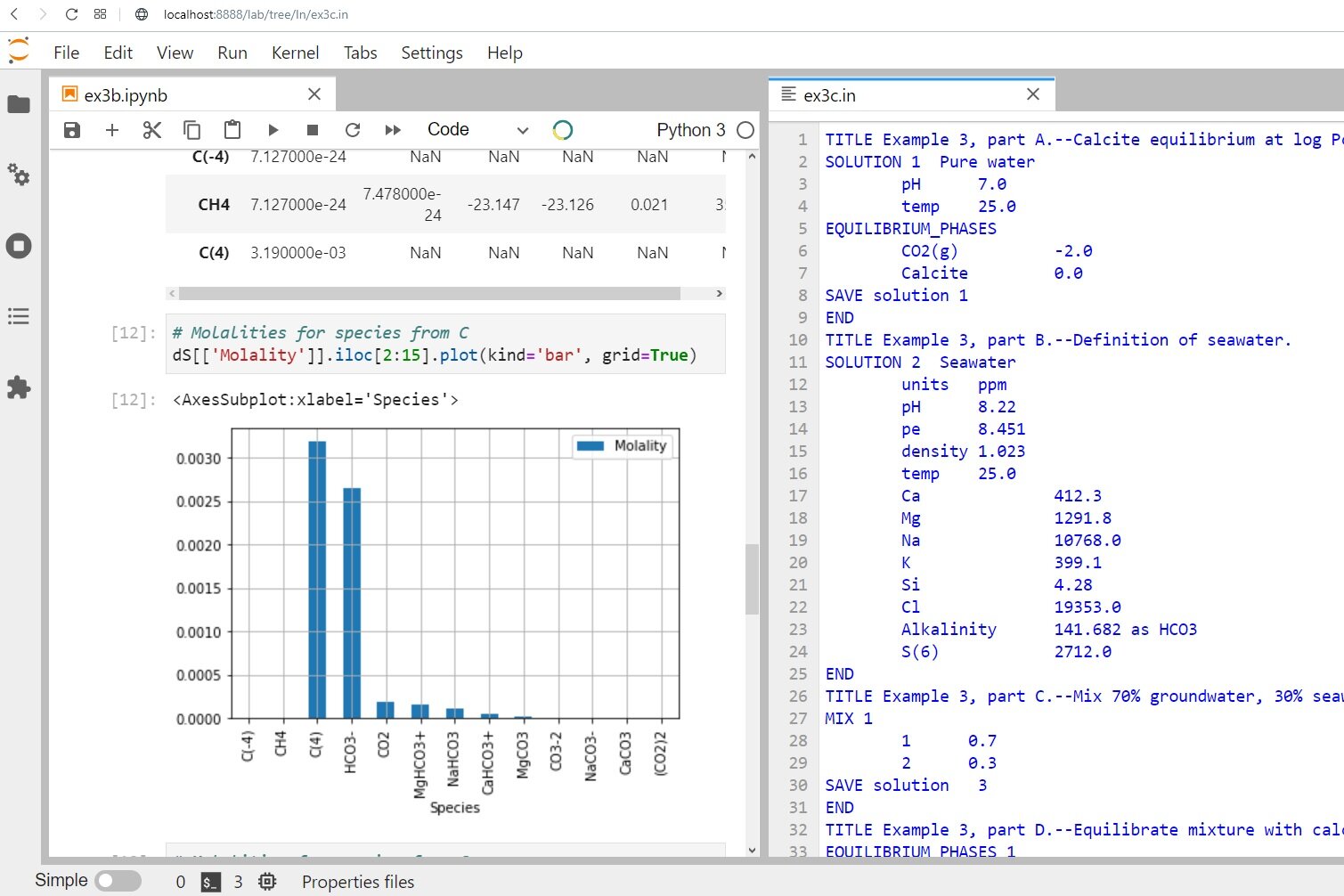
CH4	7.127000e-24	7.478000e-24	-23.147	-23.126	0.021	35.46
C(4)	3.190000e-03	NaN	NaN	NaN	NaN	NaN

# Molalities for species from C
dS[['Molality']].iloc[2:15].plot(kind='bar', grid=True)

<AxesSubplot:xlabel='Species'>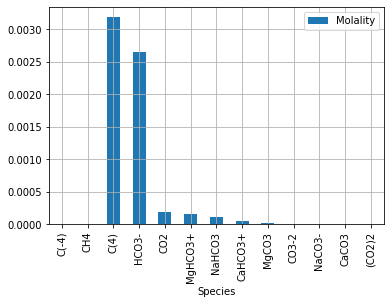

# Molalities for species from Ca
dS[['Molality']].iloc[15:22].plot(kind='bar', grid=True)

<AxesSubplot:xlabel='Species'>

sI = batchReact['saturationIndices']
sI.head()

	SI	log IAP	log K(298 K, 1 atm)	Description
Phase
Anhydrite	-1.42	-5.70	-4.28	CaSO4
Aragonite	-0.25	-8.58	-8.34	CaCO3
Calcite	-0.10	-8.58	-8.48	CaCO3
CH4(g)	-20.32	-23.13	-2.80	CH4
Chalcedony	-1.08	-4.63	-3.55	SiO2

sI[['SI']].plot(kind='bar', figsize=(12,4), grid=True)

<AxesSubplot:xlabel='Phase'>

# plot saturation values higher than -5
sI[['SI']][sI[['SI']]>-5].plot(kind='bar', figsize=(12,4), grid=True)

Datos de entrada

Puede descargar los archivos de entrada desde este enlace.