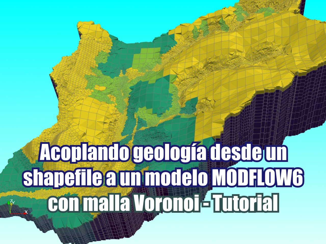
Un enfoque práctico para configurar la conductividad hidráulica en un modelo MODFLOW 6 basado en polígonos geológicos. El tutorial muestra todos los pasos desde la creación de la malla y el modelo, la configuración de los parámetros hidráulicos y la representación 3D de la distribución final en Paraview.
Tutorial
Código
from mf6Voronoi.utils import initiateOutputFolder
import flopy
from mf6Voronoi.utils import listTemplates, copyTemplate
#get the latest modflow binary
binDir = '../bin'
initiateOutputFolder(binDir)The output folder ../bin exists and has been clearedflopy.utils.get_modflow(binDir, subset=['mf6'])fetched release '23.0' info from MODFLOW-ORG/executables
using previous download 'C:\Users\saulm\Downloads\modflow_executables-23.0-win64.zip' (use 'force=True' to re-download)
extracting 1 file to 'C:\Users\saulm\Documents\howToHydraulicCondFromGeology\bin'
mf6.exe (6.6.3)
updated flopy metadata file: 'C:\Users\saulm\AppData\Local\flopy\get_modflow.json'#listTemplates()copyTemplate('generateVoronoi','geo')copyTemplate('modelCreation','geo')copyTemplate('vtkGeneration','geo')Mesh generation
Part 1 : Voronoi mesh generation
import warnings ## Org
warnings.filterwarnings('ignore') ## Org

import os, sys ## Org
import geopandas as gpd ## Org
from mf6Voronoi.geoVoronoi import createVoronoi ## Org
from mf6Voronoi.meshProperties import meshShape ## Org
from mf6Voronoi.utils import initiateOutputFolder, getVoronoiAsShp ## Org
#Create mesh object specifying the coarse mesh and the multiplier
vorMesh = createVoronoi(meshName='coupleGeology',maxRef = 250, multiplier=1, overlapping=False) ## Org
#Open limit layers and refinement definition layers
vorMesh.addLimit('basin','../shp/hatariUtils/catchment.shp') ## Org
vorMesh.addLayer('river','../shp/hatariUtils/river_basin.shp',40) ## Org
vorMesh.addLayer('gunsight','../shp/gunsightFormation.shp',80) ## Org#Generate point pair array
vorMesh.generateOrgDistVertices() ## Org
#Generate the point cloud and voronoi
vorMesh.createPointCloud() ## Org
vorMesh.generateVoronoi() ## Org
mf6Voronoi will have a web version in 2028
Follow us: |
 |
 |
 |
 |
 |
 |
/--------Layer river discretization-------/
Progressive cell size list: [40, 80, 120, 160, 200, 240] m.

/--------Layer gunsight discretization-------/
Progressive cell size list: [80, 160, 240] m.

/----Sumary of points for voronoi meshing----/
Distributed points from layers: 2
Points from layer buffers: 5478
Points from max refinement areas: 551
Points from min refinement areas: 1242
Total points inside the limit: 8355
/--------------------------------------------/

Time required for point generation: 1.97 seconds


/----Generation of the voronoi mesh----/

Time required for voronoi generation: 1.44 seconds
#Uncomment the next two cells if you have strong differences on discretization or you have encounter an FORTRAN error while running MODFLOW6vorMesh.checkVoronoiQuality(threshold=0.005)/----Performing quality verification of voronoi mesh----/
Short side on polygon: 8358 with length = 0.00036
Short side on polygon: 8358 with length = 0.00036
Short side on polygon: 8358 with length = 0.00029
Short side on polygon: 8358 with length = 0.00029
Short side on polygon: 8358 with length = 0.00194
Short side on polygon: 8358 with length = 0.00194
Short side on polygon: 8358 with length = 0.00395
Short side on polygon: 8358 with length = 0.00395vorMesh.fixVoronoiShortSides()
vorMesh.generateVoronoi()
vorMesh.checkVoronoiQuality(threshold=0.005)/----Generation of the voronoi mesh----/
Time required for voronoi generation: 1.59 seconds
/----Performing quality verification of voronoi mesh----/
Your mesh has no edges shorter than your threshold#Export generated voronoi mesh
initiateOutputFolder('../output') ## Org
getVoronoiAsShp(vorMesh.modelDis, shapePath='../output/'+vorMesh.modelDis['meshName']+'.shp') ## OrgThe output folder ../output has been generated.
/----Generation of the voronoi shapefile----/
Time required for voronoi shapefile: 1.94 seconds# Show the resulting voronoi mesh
#open the mesh file
mesh=gpd.read_file('../output/'+vorMesh.modelDis['meshName']+'.shp') ## Org
#plot the mesh
mesh.plot(figsize=(35,25), fc='crimson', alpha=0.3, ec='teal') ## Org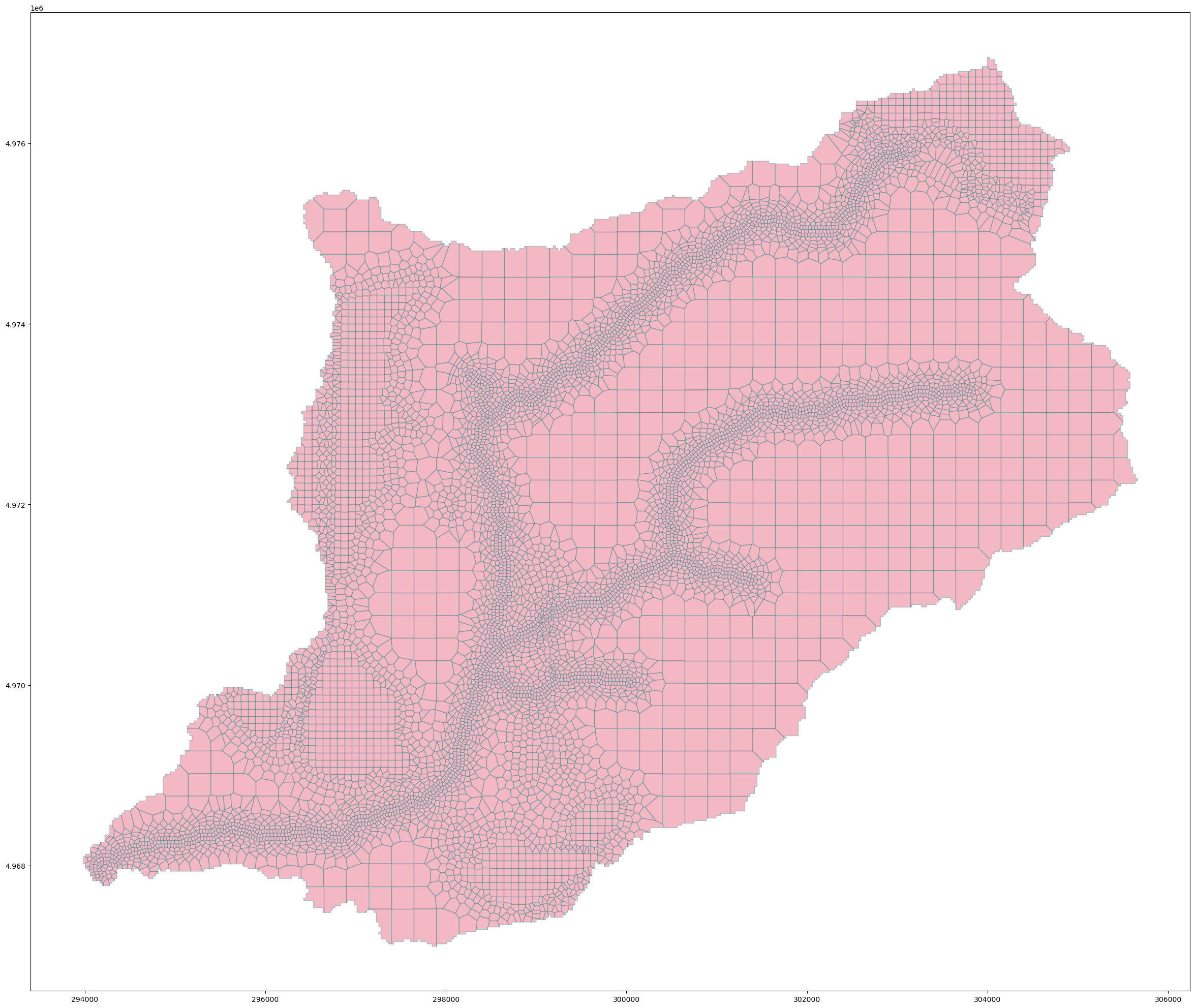
Part 2 generate disv properties
# open the mesh file
mesh=meshShape('../output/'+vorMesh.modelDis['meshName']+'.shp') ## Org
# get the list of vertices and cell2d data
gridprops=mesh.get_gridprops_disv() ## OrgCreating a unique list of vertices [[x1,y1],[x2,y2],...]
100%|███████████████████████████████████████████████████████████████████████████| 8363/8363 [00:00<00:00, 18441.82it/s]
Extracting cell2d data and grid index
100%|████████████████████████████████████████████████████████████████████████████| 8363/8363 [00:03<00:00, 2451.03it/s]#create folder
initiateOutputFolder('../json') ## Org
#export disv
mesh.save_properties('../json/disvDict.json') ## OrgThe output folder ../json has been generated.Model creation on steady state
Part 2a: generate disv properties
import sys, json, os ## Org
import rasterio, flopy ## Org
import numpy as np ## Org
import matplotlib.pyplot as plt ## Org
import geopandas as gpd ## Org
from mf6Voronoi.meshProperties import meshShape ## Org
from shapely.geometry import MultiLineString ## Org
# open the json file
with open('../json/disvDict.json') as file: ## Org
gridProps = json.load(file) ## Orgcell2d = gridProps['cell2d'] #cellid, cell centroid xy, vertex number and vertex id list
vertices = gridProps['vertices'] #vertex id and xy coordinates
ncpl = gridProps['ncpl'] #number of cells per layer
nvert = gridProps['nvert'] #number of verts
centroids=gridProps['centroids'] #cell centroids xyPart 2b: Model construction and simulation
#Extract dem values for each centroid of the voronois
src = rasterio.open('../rst/modelDem.tif')  ## Org
elevation=[x for x in src.sample(centroids)] ## Org
nlay = 15 ## Org
mtop=np.array([elev[0] for i,elev in enumerate(elevation)]) ## Org
zbot=np.zeros((nlay,ncpl)) ## Org
AcuifInf_Bottom = 1300 ## Org
zbot[0,] = AcuifInf_Bottom + (0.95 * (mtop - AcuifInf_Bottom)) ## Org
zbot[1,] = AcuifInf_Bottom + (0.9 * (mtop - AcuifInf_Bottom)) ## Org
zbot[2,] = AcuifInf_Bottom + (0.85 * (mtop - AcuifInf_Bottom)) ## Org
zbot[3,] = AcuifInf_Bottom + (0.8 * (mtop - AcuifInf_Bottom)) ## Org
zbot[4,] = AcuifInf_Bottom + (0.75 * (mtop - AcuifInf_Bottom)) ## Org
zbot[5,] = AcuifInf_Bottom + (0.7 * (mtop - AcuifInf_Bottom)) ## Org
zbot[6,] = AcuifInf_Bottom + (0.65 * (mtop - AcuifInf_Bottom)) ## Org
zbot[7,] = AcuifInf_Bottom + (0.6 * (mtop - AcuifInf_Bottom)) ## Org
zbot[8,] = AcuifInf_Bottom + (0.55 * (mtop - AcuifInf_Bottom)) ## Org
zbot[9,] = AcuifInf_Bottom + (0.5 * (mtop - AcuifInf_Bottom)) ## Org
zbot[10,] = AcuifInf_Bottom + (0.4 * (mtop - AcuifInf_Bottom)) ## Org
zbot[11,] = AcuifInf_Bottom + (0.3 * (mtop - AcuifInf_Bottom)) ## Org
zbot[12,] = AcuifInf_Bottom + (0.2 * (mtop - AcuifInf_Bottom)) ## Org
zbot[13,] = AcuifInf_Bottom + (0.1 * (mtop - AcuifInf_Bottom)) ## Org
zbot[14,] = AcuifInf_BottomCreate simulation and model
# create simulation
simName = 'mf6Sim' ## Org
modelName = 'mf6Model' ## Org
modelWs = '../modelFiles' ## Org
sim = flopy.mf6.MFSimulation(sim_name=modelName, version='mf6', ## Org
                             exe_name='../bin/mf6.exe', ## Org
                             sim_ws=modelWs) ## Org
# create tdis package
tdis_rc = [(1000.0, 1, 1.0)] ## Org
tdis = flopy.mf6.ModflowTdis(sim, pname='tdis', time_units='SECONDS', ## Org
perioddata=tdis_rc) ## Org# create gwf model
gwf = flopy.mf6.ModflowGwf(sim, ## Org
modelname=modelName, ## Org
save_flows=True, ## Org
newtonoptions="NEWTON UNDER_RELAXATION") ## Org# create iterative model solution and register the gwf model with it
ims = flopy.mf6.ModflowIms(sim, ## Org
complexity='COMPLEX', ## Org
outer_maximum=50, ## Org
inner_maximum=30, ## Org
linear_acceleration='BICGSTAB') ## Org
sim.register_ims_package(ims,[modelName]) ## Org# disv
disv = flopy.mf6.ModflowGwfdisv(gwf, nlay=nlay, ncpl=ncpl, ## Org
top=mtop, botm=zbot, ## Org
nvert=nvert, vertices=vertices, ## Org
cell2d=cell2d) ## Org# initial conditions
ic = flopy.mf6.ModflowGwfic(gwf, strt=np.stack([mtop for i in range(nlay)])) ## OrgKxArray = np.ones((nlay, ncpl)) * 4e-4
KxArray[1:6] = 5e-6
KxArray[6:15] = 3e-6
KxArray[15:] = 7e-7
icelltype = [1 for x in range(7)] + [0 for x in range(nlay - 7)]
interIx = flopy.utils.gridintersect.GridIntersect(gwf.modelgrid) ## Org
geoDf = gpd.read_file('../shp/geology.shp')
#looping over the geology polygons
for index, row in geoDf.iterrows():
geoCells=interIx.intersect(row.geometry).cellids
# for aluvial layers, that has 'alluvium' or 'deposit' on the notes
if 'alluvium' in row.Notes or 'deposits' in row.Notes:
for cell in geoCells:
KxArray[0,cell] = row.Cond #only apply to the first layer
#for the rest of layers
else:
for cell in geoCells:
KxArray[1:,cell] = row.Cond #apply to the remaining layers below layer 1
# node property flow
npf = flopy.mf6.ModflowGwfnpf(gwf, ## Org
save_specific_discharge=True, ## Org
icelltype=icelltype, ## Org
k=KxArray,
k33=KxArray/10) ## Org#cross section over the main river
crossSection = gpd.read_file('../shp/crossSection.shp') ## Org
sectionLine =list(crossSection.iloc[0].geometry.coords) ## Org
fig, ax = plt.subplots(figsize=(12,8)) ## Org
modelxsect = flopy.plot.PlotCrossSection(model=gwf, line={'Line': sectionLine}) ## Org
linecollection = modelxsect.plot_grid(lw=0.5) ## Org
modelxsect.plot_array(np.log(npf.k.array), cmap='viridis', alpha=0.5)
ax.grid() ## Org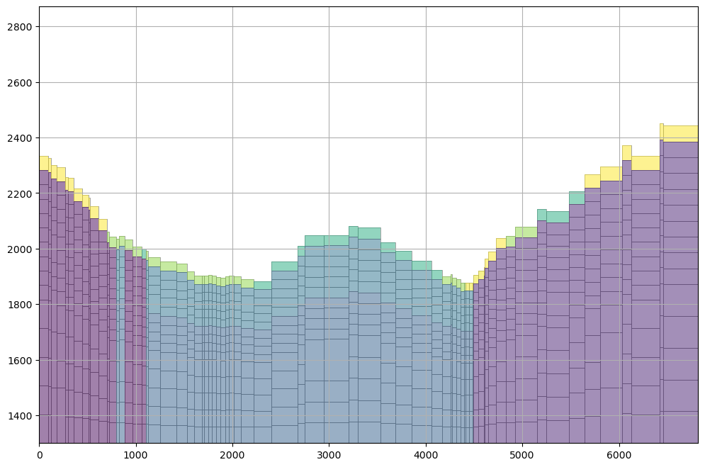
sim.write_simulation()writing simulation...
writing simulation name file...
writing simulation tdis package...
writing solution package ims_-1...
writing model mf6Model...
writing model name file...
writing package disv...
writing package ic...
writing package npf...3d geometry generation on Vtk format
#Vtk generation
import flopy ## Org
from mf6Voronoi.tools.vtkGen import Mf6VtkGenerator ## Org
from mf6Voronoi.utils import initiateOutputFolder ## Org
# load simulation
simName = 'mf6Sim' ## Org
modelName = 'mf6Model' ## Org
modelWs = '../modelFiles' ## Org
sim = flopy.mf6.MFSimulation.load(sim_name=modelName, version='mf6', ## Org
exe_name='bin/mf6.exe', ## Org
sim_ws=modelWs) ## Orgloading simulation...
loading simulation name file...
loading tdis package...
loading model gwf6...
loading package disv...
loading package ic...
loading package npf...
loading solution package mf6model...vtkDir = '../vtk' ## Org
initiateOutputFolder(vtkDir) ## Org
mf6Vtk = Mf6VtkGenerator(sim, vtkDir) ## OrgThe output folder ../vtk has been generated.mf6Voronoi will have a web version in 2028
Follow us: |
|
|
|
|
|
|
/---------------------------------------/

The Vtk generator engine has been started

/---------------------------------------/
#list models on the simulation
mf6Vtk.listModels() ## OrgModels in simulation: ['mf6model']mf6Vtk.loadModel(modelName) ## OrgPackage list: ['DISV', 'IC', 'NPF']#generate model geometry as vtk and parameter array
mf6Vtk.generateGeometryArrays() ## Org#generate parameter vtk
mf6Vtk.generateParamVtk() ## OrgParameter Vtk GeneratedDatos de ingreso
Puedes descargar los datos de ingreso desde este enlace.
owncloud.hatarilabs.com/s/PBswAAxpBCU7VyJ
Password: Hatarilabs