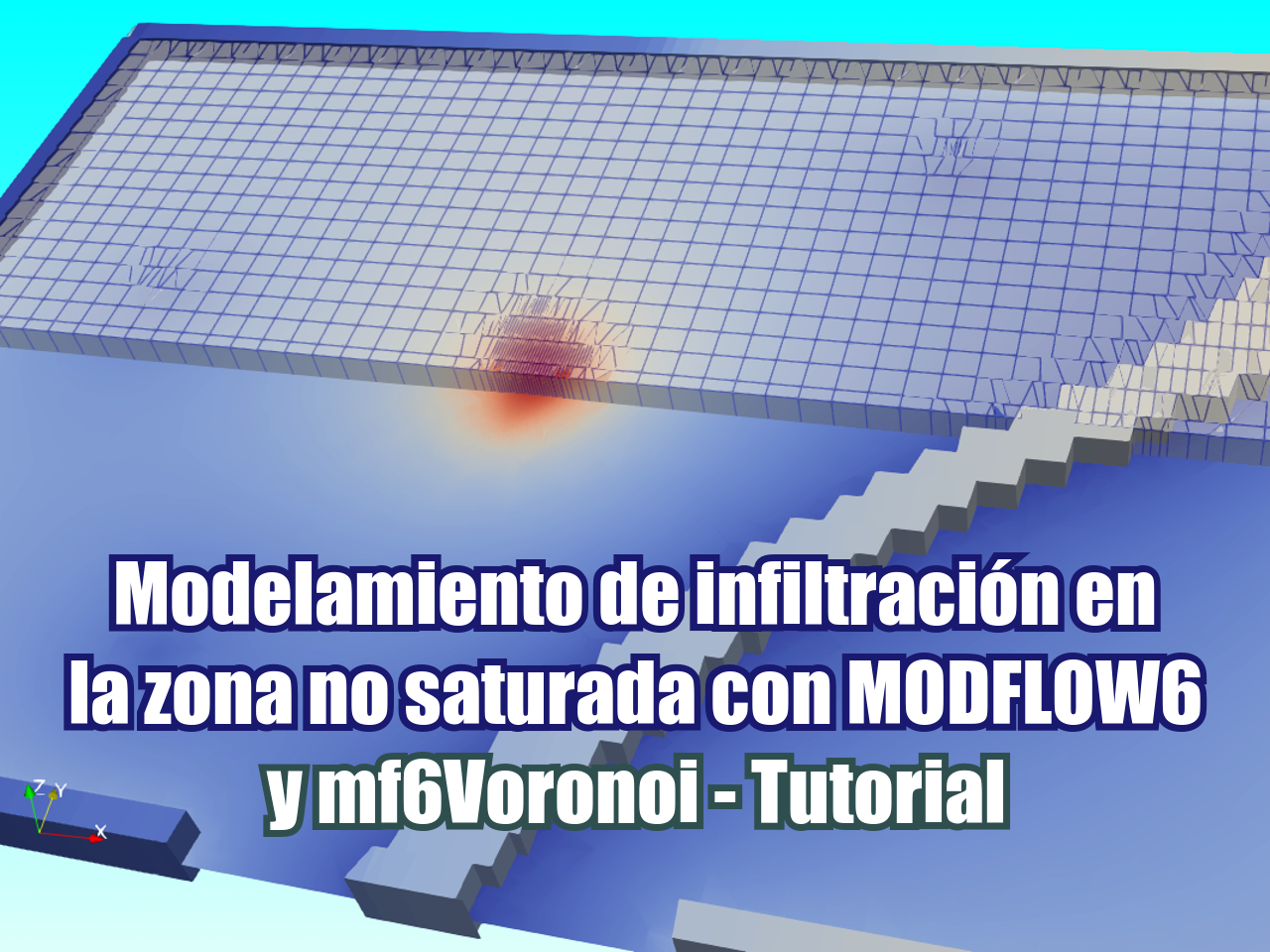
Caso aplicado de simulación de infiltración en la zona no saturada utilizando el paquete UZF de MODFLOW 6 sobre una grilla Voronoi geoespacial construida con mf6Voronoi. El modelo está en régimen uniforme y transitorio con 3 capas donde la infiltración en la zona no saturada ocurre en la primera capa. Se inserta un punto de observación con distintas profundidades para hacer una evaluación del perfil profundidad-humedad con el tiempo para las distintas tazas de infiltración; por último, se genera una representación 3D de la superficie final de la napa freática con el efecto de las condiciones de borde y la infiltración.
Tutorial
Código
from mf6Voronoi.utils import listTemplates, copyTemplate#listTemplates()copyTemplate('generateVoronoi','unsat')copyTemplate('multilayeredTransient','unsat')copyTemplate('vtkGeneration','unsat')Part 1 : Voronoi mesh generation
import warnings ## Org
warnings.filterwarnings('ignore') ## Org

import os, sys ## Org
import geopandas as gpd ## Org
from mf6Voronoi.geoVoronoi import createVoronoi ## Org
from mf6Voronoi.meshProperties import meshShape ## Org
from mf6Voronoi.utils import initiateOutputFolder, getVoronoiAsShp ## Org
#Create mesh object specifying the coarse mesh and the multiplier
vorMesh = createVoronoi(meshName='infiltrationPond',maxRef = 10, multiplier=1.5) ## Org
#Open limit layers and refinement definition layers
vorMesh.addLimit('basin','../shp/modelLimit.shp') ## <=== updated
vorMesh.addLayer('pond','../shp/infiltrationPond.shp',1) ## <=== updated
vorMesh.addLayer('regionalFlow','../shp/regionalFlow.shp',5) ## <=== updated
vorMesh.addLayer('river','../shp/river.shp',4) ## <=== updated
vorMesh.addLayer('wells','../shp/wells.shp',1) ## <=== updated#Generate point pair array
vorMesh.generateOrgDistVertices() ## Org
#Generate the point cloud and voronoi
vorMesh.createPointCloud() ## Org
vorMesh.generateVoronoi() ## Org
mf6Voronoi will have a web version in 2028
Follow us: |
 |
 |
 |
 |
 |
 |
/--------Layer pond discretization-------/
Progressive cell size list: [1, 2.5, 4.75, 8.125] m.

/--------Layer regionalFlow discretization-------/
Progressive cell size list: [5] m.

/--------Layer river discretization-------/
Progressive cell size list: [4, 10.0] m.

/--------Layer wells discretization-------/
Progressive cell size list: [1, 2.5, 4.75, 8.125] m.

/----Sumary of points for voronoi meshing----/
Distributed points from layers: 4
Points from layer buffers: 1580
Points from max refinement areas: 1419
Points from min refinement areas: 1949
Total points inside the limit: 5376
/--------------------------------------------/

Time required for point generation: 1.38 seconds


/----Generation of the voronoi mesh----/

Time required for voronoi generation: 0.60 seconds
#Uncomment the next two cells if you have strong differences on discretization or you have encounter an FORTRAN error while running MODFLOW6vorMesh.checkVoronoiQuality(threshold=0.005)/----Performing quality verification of voronoi mesh----/
Short side on polygon: 4625 with length = 0.00084
Short side on polygon: 4625 with length = 0.00084
Short side on polygon: 4625 with length = 0.00084
Short side on polygon: 4625 with length = 0.00084
Short side on polygon: 4625 with length = 0.00398
Short side on polygon: 4625 with length = 0.00398
Short side on polygon: 4625 with length = 0.00155
Short side on polygon: 4625 with length = 0.00155
Short side on polygon: 4625 with length = 0.00016
Short side on polygon: 4625 with length = 0.00158
Short side on polygon: 4625 with length = 0.00158
Short side on polygon: 4625 with length = 0.00016
Short side on polygon: 4625 with length = 0.00241
Short side on polygon: 4625 with length = 0.00241
Short side on polygon: 4625 with length = 0.00084
Short side on polygon: 4625 with length = 0.00084
Short side on polygon: 4625 with length = 0.00000
Short side on polygon: 4625 with length = 0.00000
Short side on polygon: 4625 with length = 0.00089
Short side on polygon: 4625 with length = 0.00089vorMesh.fixVoronoiShortSides()
vorMesh.generateVoronoi()
vorMesh.checkVoronoiQuality(threshold=0.005)/----Generation of the voronoi mesh----/
Time required for voronoi generation: 0.49 seconds
/----Performing quality verification of voronoi mesh----/
Your mesh has no edges shorter than your threshold#Export generated voronoi mesh
initiateOutputFolder('../output') ## Org
getVoronoiAsShp(vorMesh.modelDis, shapePath='../output/'+vorMesh.modelDis['meshName']+'.shp') ## OrgThe output folder ../output exists and has been cleared
/----Generation of the voronoi shapefile----/
Time required for voronoi shapefile: 1.06 seconds# Show the resulting voronoi mesh
#open the mesh file
mesh=gpd.read_file('../output/'+vorMesh.modelDis['meshName']+'.shp') ## Org
#plot the mesh
mesh.plot(figsize=(35,25), fc='crimson', alpha=0.3, ec='teal') ## Org
Part 2 generate disv properties
# open the mesh file
mesh=meshShape('../output/'+vorMesh.modelDis['meshName']+'.shp') ## Org
# get the list of vertices and cell2d data
gridprops=mesh.get_gridprops_disv() ## OrgCreating a unique list of vertices [[x1,y1],[x2,y2],...]
100%|███████████████████████████████████████████████████████████████████████████| 4637/4637 [00:00<00:00, 19635.21it/s]
Extracting cell2d data and grid index
100%|████████████████████████████████████████████████████████████████████████████| 4637/4637 [00:01<00:00, 3457.82it/s]#create folder
initiateOutputFolder('../json') ## Org
#export disv
mesh.save_properties('../json/disvDict.json') ## OrgThe output folder ../json exists and has been clearedPart 2a: generate disv properties
import sys, json, os ## Org
import rasterio, flopy ## Org
import numpy as np ## Org
import matplotlib.pyplot as plt ## Org
import geopandas as gpd ## Org
from mf6Voronoi.meshProperties import meshShape ## Org
from shapely.geometry import MultiLineString ## Org
from mf6Voronoi.tools.cellWork import getLayCellElevTupleFromRaster, getLayCellElevTupleFromElev
# open the json file
with open('../json/disvDict.json') as file: ## Org
gridProps = json.load(file) ## Orgcell2d = gridProps['cell2d'] #cellid, cell centroid xy, vertex number and vertex id list
vertices = gridProps['vertices'] #vertex id and xy coordinates
ncpl = gridProps['ncpl'] #number of cells per layer
nvert = gridProps['nvert'] #number of verts
centroids=gridProps['centroids'] #cell centroids xyPart 2b: Model construction and simulation
#Extract dem values for each centroid of the voronois
#src = rasterio.open('rst/elevWgs18S.tif')  ## Org
#elevation=[x for x in src.sample(centroids)] ## Org
nlay = 3 ## Org
mtop=np.array([50 for i in range(ncpl)]) ## <=== updated
zbot=np.zeros((nlay,ncpl)) ## <=== updated
zbot[0,] = [30 for i in range(ncpl)] ## <=== updated
zbot[1,] = [10 for i in range(ncpl)] ## <=== updated
zbot[2,] = [-10 for i in range(ncpl)] ## <=== updatedCreate simulation and model
# create simulation
simName = 'mf6Sim' ## Org
modelName = 'mf6Model' ## Org
modelWs = '../modelFiles' ## Org
sim = flopy.mf6.MFSimulation(sim_name=modelName, version='mf6', ## Org
                             exe_name='../bin/mf6.exe', ## Org
                             sim_ws=modelWs) ## Org
# create tdis package
tdis_rc = [(1.0, 1, 1.0)] + [(86400*10, 5, 1.5) for level in range(2)] ## Org
print(tdis_rc[:3]) ## Org
tdis = flopy.mf6.ModflowTdis(sim, pname='tdis', time_units='SECONDS', ## Org
perioddata=tdis_rc, ## Org
nper=3) ## Org[(1.0, 1, 1.0), (864000, 5, 1.5), (864000, 5, 1.5)]# create gwf model
gwf = flopy.mf6.ModflowGwf(sim, ## Org
modelname=modelName, ## Org
save_flows=True, ## Org
newtonoptions="NEWTON UNDER_RELAXATION") ## Org# create iterative model solution and register the gwf model with it
ims = flopy.mf6.ModflowIms(sim, ## Org
complexity='COMPLEX', ## Org
outer_maximum=150, ## Org
inner_maximum=50, ## Org
outer_dvclose=0.1, ## Org
inner_dvclose=0.0001, ## Org
backtracking_number=20, ## Org
linear_acceleration='BICGSTAB') ## Org
sim.register_ims_package(ims,[modelName]) ## Org# disv
disv = flopy.mf6.ModflowGwfdisv(gwf, nlay=nlay, ncpl=ncpl, ## Org
top=mtop, botm=zbot, ## Org
nvert=nvert, vertices=vertices, ## Org
cell2d=cell2d) ## Orgdisv.top.plot(figsize=(12,8), alpha=0.8) ## Org<Axes: title={'center': 'top'}>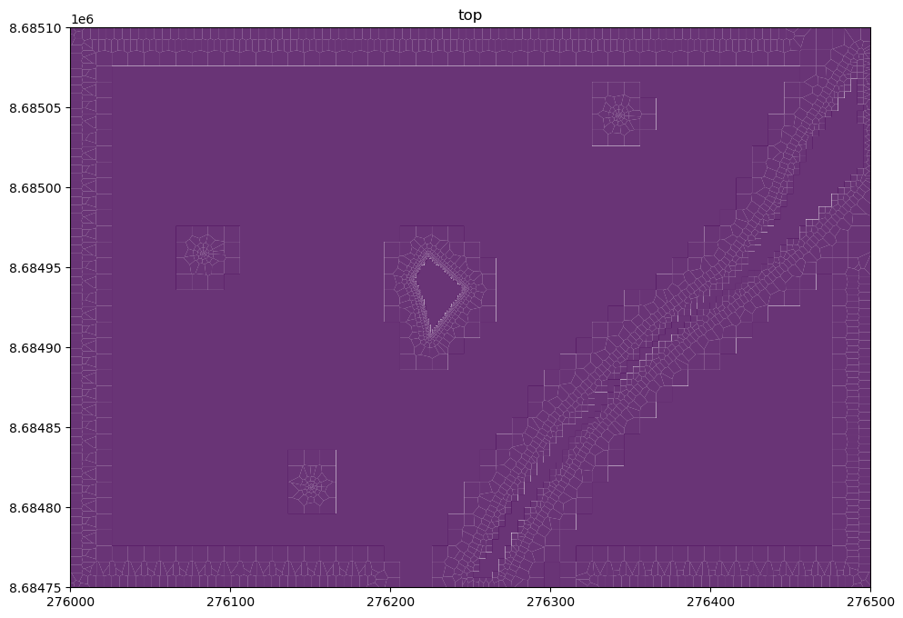
crossSection = gpd.read_file('../shp/crossSectionTotal.shp') ## Org
sectionLine =list(crossSection.iloc[0].geometry.coords) ## Org

fig, ax = plt.subplots(figsize=(12,8)) ## Org
modelxsect = flopy.plot.PlotCrossSection(model=gwf, line={'Line': sectionLine}) ## Org
linecollection = modelxsect.plot_grid(lw=0.5) ## Org
ax.grid() ## Org
# initial conditions

ic = flopy.mf6.ModflowGwfic(gwf, strt=np.stack([40 for i in range(nlay)])) ## Org
#headsInitial = np.load('npy/headCalibInitial.npy')
#ic = flopy.mf6.ModflowGwfic(gwf, strt=headsInitial)
Kx =[3E-5 for x in range(3)] ## <=== updated
icelltype = [1, 0, 0] ## <=== updated
# node property flow
npf = flopy.mf6.ModflowGwfnpf(gwf, ## Org
save_specific_discharge=True, ## Org
icelltype=icelltype, ## Org
k=Kx, ## Org
k33=Kx) ## Org# define storage and transient stress periods
sto = flopy.mf6.ModflowGwfsto(gwf, ## Org
iconvert=1, ## Org
steady_state={ ## Org
0:True, ## Org
},
transient={
1:True, ## Org
2:True, ## Org
},
ss=1e-06,
sy=0.001,
) ## OrgWorking with rechage, evapotranspiration
rchr = 0.2/365/86400 ## Org
rch = flopy.mf6.ModflowGwfrcha(gwf, recharge=rchr) ## Org
evtr = 1.2/365/86400 ## Org
evt = flopy.mf6.ModflowGwfevta(gwf,ievt=1,surface=mtop,rate=evtr,depth=1.0) ## Org
Definition of the intersect object
For the manipulation of spatial data to determine hydraulic parameters or boundary conditions
# Define intersection object
interIx = flopy.utils.gridintersect.GridIntersect(gwf.modelgrid) ## Org
#river package
layCellTupleList = getLayCellElevTupleFromElev(gwf,interIx,39.5,'../shp/river.shp') ## <=== updated
riverSpd = {} ## Org
riverSpd[0] = [] ## Org
for index, layCellTuple in enumerate(layCellTupleList): ## Org
riverSpd[0].append([layCellTuple,39.5,0.01,38]) ## Org
riverSpd[0][:5]You have inserted a fixed elevation
[[(0, 2289), 39.5, 0.01, 38],
[(0, 2452), 39.5, 0.01, 38],
[(0, 2493), 39.5, 0.01, 38],
[(0, 2528), 39.5, 0.01, 38],
[(0, 2533), 39.5, 0.01, 38]]riv = flopy.mf6.ModflowGwfriv(gwf, stress_period_data=riverSpd) ## Org#river plot
riv.plot(mflay=0, kper=1) ## Org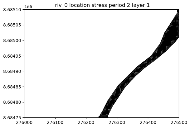
crossSection = gpd.read_file('../shp/crossSectionTotal.shp') ## Org
sectionLine =list(crossSection.iloc[0].geometry.coords) ## Org

fig, ax = plt.subplots(figsize=(12,8)) ## Org
xsect = flopy.plot.PlotCrossSection(model=gwf, line={'Line': sectionLine}) ## Org
lc = xsect.plot_grid(lw=0.5) ## Org
xsect.plot_bc('RIV',kper=2) ## Org
ax.grid() ## Org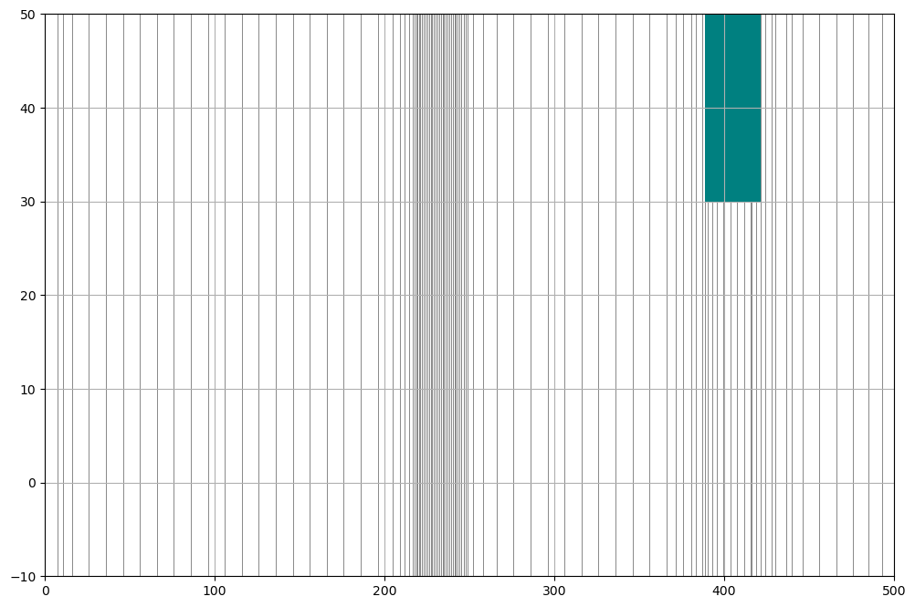
#regional flow package
layCellTupleList = getLayCellElevTupleFromElev(gwf,interIx,40,'../shp/regionalFlow.shp') ## <=== updated
ghbSpd = {} ## Org
ghbSpd[0] = [] ## Org
for index, layCellTuple in enumerate(layCellTupleList): ## <=== updated
    ghbSpd[0].append([layCellTuple,40,0.01]) ## <=== updated
ghbSpd[0][:5] ## <=== updated
You have inserted a fixed elevation
[[(0, 8), 40, 0.01],
[(0, 204), 40, 0.01],
[(0, 205), 40, 0.01],
[(0, 234), 40, 0.01],
[(0, 238), 40, 0.01]]ghb = flopy.mf6.ModflowGwfghb(gwf, stress_period_data=ghbSpd)
#regional flow plot
ghb.plot(mflay=0, kper=0) ## <===== modified
#well package
layCellTupleList = getLayCellElevTupleFromElev(gwf,interIx,20,'../shp/wells.shp') ## <=== updated
welSpd = {} ## Org
welSpd[0] = [] ## Org
for index, layCellTuple in enumerate(layCellTupleList): ## <=== updated
    welSpd[0].append([layCellTuple,-0.001]) ## <=== updated
welSpd[0][:5] ## <=== updated
You have inserted a fixed elevation
[[(1, 505), -0.001], [(1, 3286), -0.001], [(1, 825), -0.001]]wel = flopy.mf6.ModflowGwfwel(gwf, stress_period_data=welSpd)
#regional flow plot
wel.plot(mflay=1, kper=0, ec='crimson') ## <===== modified
#well package
layCellTupleListUzf = getLayCellElevTupleFromElev(gwf,interIx,40,'../shp/piezometer.shp') ## <=== updated
print(layCellTupleListUzf)
piezoCell = layCellTupleListUzf[0][1]
You have inserted a fixed elevation
[(0, 1906)]layCellTupleList = getLayCellElevTupleFromElev(gwf,interIx,50,'../shp/infiltrationPond.shp') ## <=== updated
packageData = []
for index, layCellTuple in enumerate(layCellTupleList): ## <=== updated
if layCellTuple[1] == piezoCell:
packageData.append([index, layCellTuple, 1, 0, 0.1, 3e-5, 0.1, 0.35, 0.15, 3.5,'surfRate'+str(piezoCell)]) ## <=== updated
else:
packageData.append([index, layCellTuple, 1, 0, 0.1, 3e-5, 0.1, 0.35, 0.15, 3.5,'surfRate']) ## <=== updatedYou have inserted a fixed elevationperiodData = {}
periodData[0] = []
periodData[1] = []
periodData[2] = []
for index, layCellTuple in enumerate(layCellTupleList): ## <=== updated
periodData[0].append([index, 1.11e-06, 5e-08, 1.5, 0.1, 0, 0, 0])
periodData[1].append([index, 1.67e-06, 5e-08, 1.5, 0.1, 0, 0, 0])
periodData[2].append([index, 2.68e-06, 5e-08, 1.5, 0.1, 0, 0, 0])# Create UZF package and parameters
uzf = flopy.mf6.ModflowGwfuzf(gwf,
ntrailwaves=7,
nwavesets=40,
simulate_et=True,
simulate_gwseep=False,
packagedata=packageData,
perioddata=periodData,
wc_filerecord='uzf.out',
boundnames=True)
# Observation package for Drain
uzfDict = { # <===== Inserted
"{}.uzf.obs.csv".format(modelName): [ # <===== Inserted
("wc_0.2", "water-content", "surfRate"+str(piezoCell), 0.2), # <===== Inserted
("wc_0.5", "water-content", "surfRate"+str(piezoCell), 0.5), # <===== Inserted
("wc_1", "water-content", "surfRate"+str(piezoCell), 1), # <===== Inserted
("wc_1.5", "water-content", "surfRate"+str(piezoCell), 1.5), # <===== Inserted
("wc_2", "water-content", "surfRate"+str(piezoCell), 2), # <===== Inserted
("wc_3", "water-content", "surfRate"+str(piezoCell), 3), # <===== Inserted
("wc_4", "water-content", "surfRate"+str(piezoCell), 4), # <===== Inserted
("wc_5", "water-content", "surfRate"+str(piezoCell), 5), # <===== Inserted
("wc_6", "water-content", "surfRate"+str(piezoCell), 6), # <===== Inserted
("wc_7", "water-content", "surfRate"+str(piezoCell), 7), # <===== Inserted
("wc_8", "water-content", "surfRate"+str(piezoCell), 8), # <===== Inserted
("wc_9", "water-content", "surfRate"+str(piezoCell), 9), # <===== Inserted
] # <===== Inserted
} # <===== Inserted
# Attach observation package to DRN package
uzf.obs.initialize( # <===== Inserted
filename=gwf.name+".uzf.obs", # <===== Inserted
digits=10, # <===== Inserted
print_input=True, # <===== Inserted
continuous=uzfDict # <===== Inserted
) # <===== InsertedSet the Output Control and run simulation
#oc
head_filerecord = f"{gwf.name}.hds" ## Org
budget_filerecord = f"{gwf.name}.cbc" ## Org
oc = flopy.mf6.ModflowGwfoc(gwf, ## Org
                            head_filerecord=head_filerecord, ## Org
                            budget_filerecord = budget_filerecord, ## Org
                            saverecord=[("HEAD", "LAST"),("BUDGET","LAST")]) ## Org
# Run the simulation
sim.write_simulation() ## Org
success, buff = sim.run_simulation() ## Orgwriting simulation...
writing simulation name file...
writing simulation tdis package...
writing solution package ims_-1...
writing model mf6Model...
writing model name file...
writing package disv...
writing package ic...
writing package npf...
writing package sto...
writing package rcha_0...
writing package evta_0...
writing package riv_0...
INFORMATION: maxbound in ('gwf6', 'riv', 'dimensions') changed to 1574 based on size of stress_period_data
writing package ghb_0...
INFORMATION: maxbound in ('gwf6', 'ghb', 'dimensions') changed to 269 based on size of stress_period_data
writing package wel_0...
INFORMATION: maxbound in ('gwf6', 'wel', 'dimensions') changed to 3 based on size of stress_period_data
writing package uzf_0...
INFORMATION: nuzfcells in ('gwf6', 'uzf', 'dimensions') changed to 964 based on size of packagedata
writing package obs_0...
writing package oc...
FloPy is using the following executable to run the model: ..\bin\mf6.exe
MODFLOW 6
U.S. GEOLOGICAL SURVEY MODULAR HYDROLOGIC MODEL
VERSION 6.6.0 12/20/2024
MODFLOW 6 compiled Dec 31 2024 17:10:16 with Intel(R) Fortran Intel(R) 64
Compiler Classic for applications running on Intel(R) 64, Version 2021.7.0
Build 20220726_000000
This software has been approved for release by the U.S. Geological
Survey (USGS). Although the software has been subjected to rigorous
review, the USGS reserves the right to update the software as needed
pursuant to further analysis and review. No warranty, expressed or
implied, is made by the USGS or the U.S. Government as to the
functionality of the software and related material nor shall the
fact of release constitute any such warranty. Furthermore, the
software is released on condition that neither the USGS nor the U.S.
Government shall be held liable for any damages resulting from its
authorized or unauthorized use. Also refer to the USGS Water
Resources Software User Rights Notice for complete use, copyright,
and distribution information.
MODFLOW runs in SEQUENTIAL mode
Run start date and time (yyyy/mm/dd hh:mm:ss): 2025/08/21 17:29:26
Writing simulation list file: mfsim.lst
Using Simulation name file: mfsim.nam
Solving: Stress period: 1 Time step: 1
Solving: Stress period: 2 Time step: 1
Solving: Stress period: 2 Time step: 2
Solving: Stress period: 2 Time step: 3
Solving: Stress period: 2 Time step: 4
Solving: Stress period: 2 Time step: 5
Solving: Stress period: 3 Time step: 1
Solving: Stress period: 3 Time step: 2
Solving: Stress period: 3 Time step: 3
Solving: Stress period: 3 Time step: 4
Solving: Stress period: 3 Time step: 5
Run end date and time (yyyy/mm/dd hh:mm:ss): 2025/08/21 17:29:29
Elapsed run time: 3.652 Seconds
Normal termination of simulation.Model output visualization
headObj = gwf.output.head() ## Org
headObj.get_kstpkper() ## Org
[(np.int32(0), np.int32(0)),
(np.int32(4), np.int32(1)),
(np.int32(4), np.int32(2))]kper = 2 ## Org
lay = 0 ## Orgheads = headObj.get_data(kstpkper=(4,kper))
#heads[lay,0,:5]
#heads = headObj.get_data(kstpkper=(0,0))
#np.save('npy/headCalibInitial', heads)### Plot the heads for a defined layer and boundary conditions
fig = plt.figure(figsize=(12,8)) ## Org
ax = fig.add_subplot(1, 1, 1, aspect='equal') ## Org
modelmap = flopy.plot.PlotMapView(model=gwf) ## Org
####
levels = np.linspace(heads[heads>-1e+30].min(),heads[heads>-1e+30].max(),num=10) ## Org
contour = modelmap.contour_array(heads[lay],ax=ax,levels=levels,cmap='PuBu')
ax.clabel(contour) ## Org
quadmesh = modelmap.plot_bc('RIV') ## Org
cellhead = modelmap.plot_array(heads[lay],ax=ax, cmap='Blues', alpha=0.8)
linecollection = modelmap.plot_grid(linewidth=0.3, alpha=0.5, color='cyan', ax=ax) ## Org
plt.colorbar(cellhead, shrink=0.75) ## Org
plt.show() ## Org
crossSection = gpd.read_file('../shp/crossSectionTotal.shp')
sectionLine =list(crossSection.iloc[0].geometry.coords)

waterTable = flopy.utils.postprocessing.get_water_table(heads)

fig, ax = plt.subplots(figsize=(12,8))
xsect = flopy.plot.PlotCrossSection(model=gwf, line={'Line': sectionLine})
lc = modelxsect.plot_grid(lw=0.5)
xsect.plot_array(heads, alpha=0.5)
xsect.plot_surface(waterTable)
xsect.plot_bc('riv', kper=kper, facecolor='none', edgecolor='teal')
plt.show()
#Vtk generation
import flopy ## Org
from mf6Voronoi.tools.vtkGen import Mf6VtkGenerator ## Org
from mf6Voronoi.utils import initiateOutputFolder ## Org
# load simulation
simName = 'mf6Sim' ## Org
modelName = 'mf6Model' ## Org
modelWs = '../modelFiles' ## Org
sim = flopy.mf6.MFSimulation.load(sim_name=modelName, version='mf6', ## Org
exe_name='bin/mf6.exe', ## Org
sim_ws=modelWs) ## Orgloading simulation...
loading simulation name file...
loading tdis package...
loading model gwf6...
loading package disv...
loading package ic...
loading package npf...
loading package sto...
loading package rch...
loading package evt...
loading package riv...
loading package ghb...
loading package wel...
loading package uzf...
loading package oc...
loading solution package mf6model...vtkDir = '../vtk' ## Org
initiateOutputFolder(vtkDir) ## Org
mf6Vtk = Mf6VtkGenerator(sim, vtkDir) ## OrgThe output folder ../vtk has been generated.mf6Voronoi will have a web version in 2028
Follow us: |
|
|
|
|
|
|
/---------------------------------------/

The Vtk generator engine has been started

/---------------------------------------/
#list models on the simulation
mf6Vtk.listModels() ## OrgModels in simulation: ['mf6model']mf6Vtk.loadModel(modelName) ## OrgPackage list: ['DISV', 'IC', 'NPF', 'STO', 'RCHA_0', 'EVTA_0', 'RIV_0', 'GHB_0', 'WEL_0', 'UZF_OBS', 'UZF_0', 'OC']#show output data
headObj = mf6Vtk.gwf.output.head() ## Org
headObj.get_kstpkper() ## Org[(np.int32(0), np.int32(0)),
(np.int32(4), np.int32(1)),
(np.int32(4), np.int32(2))]#generate model geometry as vtk and parameter array
mf6Vtk.generateGeometryArrays() ## Org#generate parameter vtk
mf6Vtk.generateParamVtk() ## OrgParameter Vtk Generated#generate bc and obs vtk
mf6Vtk.generateBcObsVtk(nper=0, skipList=['UZF_0']) ## Org/--------RCHA_0 vtk generation-------/
Working for RCHA_0 package, creating the datasets: dict_keys(['irch', 'recharge', 'aux'])
Vtk file took 0.0717 seconds to be generated.
/--------RCHA_0 vtk generated-------/
/--------EVTA_0 vtk generation-------/
Working for EVTA_0 package, creating the datasets: dict_keys(['ievt', 'surface', 'rate', 'depth', 'aux'])
Vtk file took 0.0717 seconds to be generated.
/--------EVTA_0 vtk generated-------/
/--------RIV_0 vtk generation-------/
Working for RIV_0 package, creating the datasets: ('stage', 'cond', 'rbot')
Vtk file took 5.3350 seconds to be generated.
/--------RIV_0 vtk generated-------/
/--------GHB_0 vtk generation-------/
Working for GHB_0 package, creating the datasets: ('bhead', 'cond')
Vtk file took 0.7605 seconds to be generated.
/--------GHB_0 vtk generated-------/
/--------WEL_0 vtk generation-------/
Working for WEL_0 package, creating the datasets: ('q',)
Vtk file took 0.0358 seconds to be generated.
/--------WEL_0 vtk generated-------/mf6Vtk.generateHeadVtk(nper=2, nstp=4, crop=True) ## Orgmf6Vtk.generateWaterTableVtk(nper=2, nstp=4) ## Orgimport flopy
import flopy.utils.binaryfile as bf
import pandas as pd
import matplotlib.pyplot as plthead_file_path = '../modelFiles/uzf.out'wobj = flopy.utils.HeadFile(head_file_path, text="WATER-CONTENT")
wc = wobj.get_alldata()wc[2][0][0][:5]array([0.12709341, 0.22359167, 0.22358948, 0.22358385, 0.22358763])uzfDf = pd.read_csv('../modelFiles/mf6Model.uzf.obs.csv', index_col=0)
uzfDf.head()| WC_0.2 | WC_0.5 | WC_1 | WC_1.5 | WC_2 | WC_3 | WC_4 | WC_5 | WC_6 | WC_7 | WC_8 | WC_9 | |
|---|---|---|---|---|---|---|---|---|---|---|---|---|
| time | ||||||||||||
| 1.000000 | 0.150000 | 0.150000 | 0.150000 | 0.150000 | 0.150000 | 0.150000 | 0.150000 | 0.150000 | 0.150000 | 0.150000 | 0.150000 | 0.150000 |
| 65517.587678 | 0.207348 | 0.207348 | 0.207348 | 0.208439 | 0.150000 | 0.150000 | 0.150000 | 0.150000 | 0.150000 | 0.150000 | 0.150000 | 0.150000 |
| 163792.469194 | 0.206256 | 0.206256 | 0.206256 | 0.207893 | 0.209531 | 0.209531 | 0.209531 | 0.150000 | 0.150000 | 0.150000 | 0.150000 | 0.150000 |
| 311204.791469 | 0.204618 | 0.204618 | 0.204618 | 0.207075 | 0.209531 | 0.209531 | 0.209531 | 0.209531 | 0.209531 | 0.209531 | 0.206256 | 0.150000 |
| 532323.274882 | 0.202161 | 0.202161 | 0.202161 | 0.205846 | 0.209531 | 0.209531 | 0.209531 | 0.209531 | 0.209531 | 0.209531 | 0.209531 | 0.209531 |
uzfDf.index = uzfDf.index / 86400
uzfDf.index.name = 'time(days)'
uzfTr = uzfDf.transpose()
uzfTr.head()| time(days) | 0.000012 | 0.758305 | 1.895746 | 3.601907 | 6.161149 | 10.000012 | 10.758305 | 11.895746 | 13.601907 | 16.161149 | 20.000012 |
|---|---|---|---|---|---|---|---|---|---|---|---|
| WC_0.2 | 0.15 | 0.207348 | 0.206256 | 0.204618 | 0.202161 | 0.198475 | 0.223196 | 0.222105 | 0.220467 | 0.218010 | 0.214324 |
| WC_0.5 | 0.15 | 0.207348 | 0.206256 | 0.204618 | 0.202161 | 0.198475 | 0.223196 | 0.222105 | 0.220467 | 0.218010 | 0.214324 |
| WC_1 | 0.15 | 0.207348 | 0.206256 | 0.204618 | 0.202161 | 0.198475 | 0.223196 | 0.222105 | 0.220467 | 0.218010 | 0.214324 |
| WC_1.5 | 0.15 | 0.208439 | 0.207893 | 0.207075 | 0.205846 | 0.204003 | 0.224288 | 0.223742 | 0.222924 | 0.221695 | 0.219852 |
| WC_2 | 0.15 | 0.150000 | 0.209531 | 0.209531 | 0.209531 | 0.209531 | 0.225380 | 0.225380 | 0.225380 | 0.225380 | 0.225380 |
depthValues = [float(x.split('_')[1]) for x in uzfTr.index.values.tolist()]
uzfTr['depth'] = depthValues
uzfTr = uzfTr.set_index('depth')
uzfTr.head()| time(days) | 0.000012 | 0.758305 | 1.895746 | 3.601907 | 6.161149 | 10.000012 | 10.758305 | 11.895746 | 13.601907 | 16.161149 | 20.000012 |
|---|---|---|---|---|---|---|---|---|---|---|---|
| depth | |||||||||||
| 0.2 | 0.15 | 0.207348 | 0.206256 | 0.204618 | 0.202161 | 0.198475 | 0.223196 | 0.222105 | 0.220467 | 0.218010 | 0.214324 |
| 0.5 | 0.15 | 0.207348 | 0.206256 | 0.204618 | 0.202161 | 0.198475 | 0.223196 | 0.222105 | 0.220467 | 0.218010 | 0.214324 |
| 1.0 | 0.15 | 0.207348 | 0.206256 | 0.204618 | 0.202161 | 0.198475 | 0.223196 | 0.222105 | 0.220467 | 0.218010 | 0.214324 |
| 1.5 | 0.15 | 0.208439 | 0.207893 | 0.207075 | 0.205846 | 0.204003 | 0.224288 | 0.223742 | 0.222924 | 0.221695 | 0.219852 |
| 2.0 | 0.15 | 0.150000 | 0.209531 | 0.209531 | 0.209531 | 0.209531 | 0.225380 | 0.225380 | 0.225380 | 0.225380 | 0.225380 |
fig, ax = plt.subplots()
for key in uzfTr.keys():
    ax.plot(uzfTr[key], uzfTr.index, label='T: %.2f days'%key, alpha=0.5)
ax.invert_yaxis()
ax.set_xlabel('water content %')
ax.set_ylabel('depth (m)')
ax.legend()
Datos de entrada
Puedes descargar los datos de entrada desde este link:
https://owncloud.hatarilabs.com/s/4PPFzv6HW8xI315
Password: Hatarilabs