Cómo graficar niveles de agua de un modelo bidimensional en HEC-RAS usando Python - Tutorial

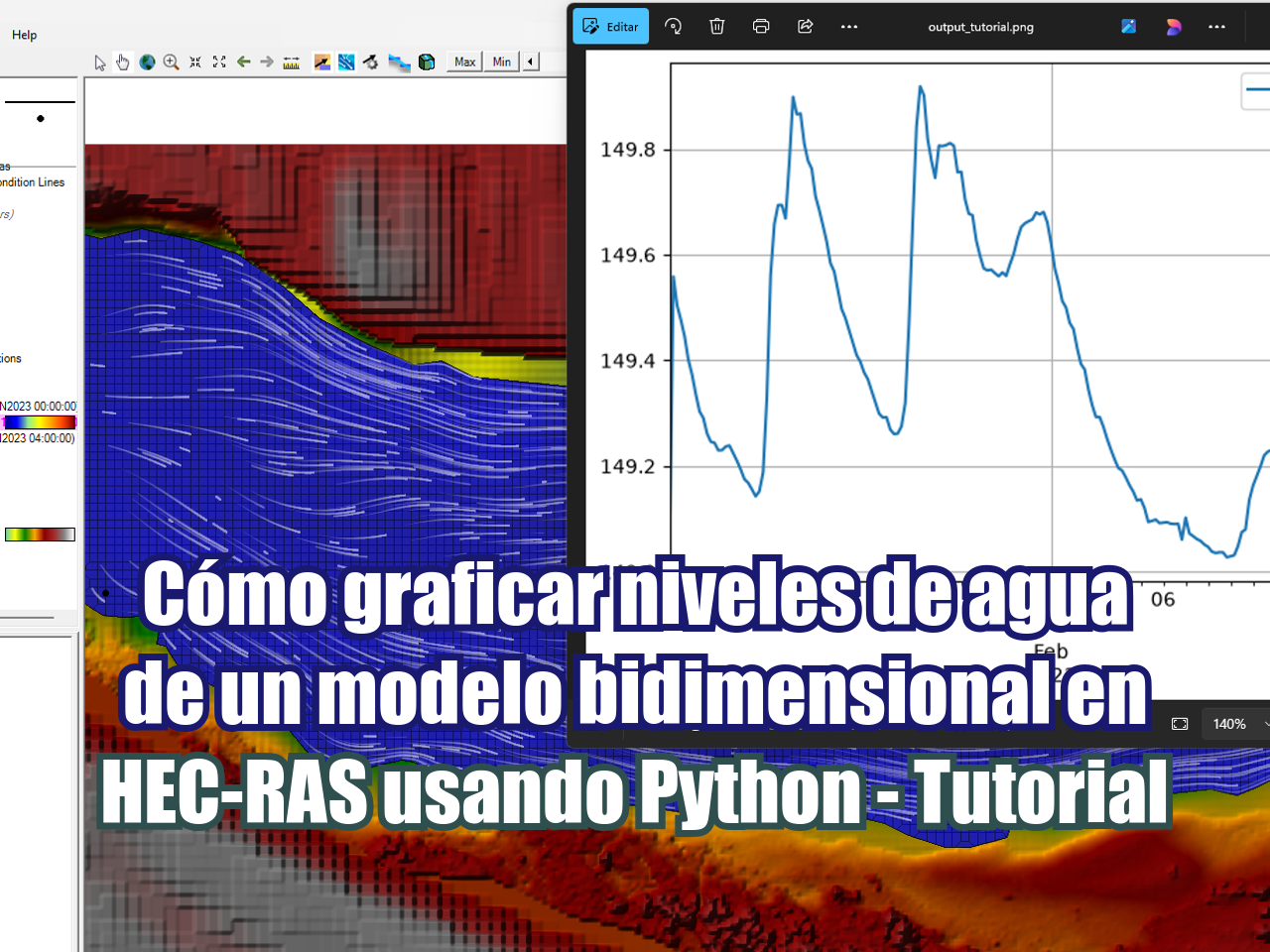
En este tutorial se explica cómo extraer de forma precisa y eficiente la superficie del agua en un punto específico de un modelo bidimensional en tránsito de HEC-RAS utilizando Python dentro del entorno de Jupyter Lab. Debido a que los niveles de agua varían a lo largo del mallado y las herramientas nativas del software a veces limitan la automatización, este tutorial enseña a abrir los archivos de salida HDF5 (.hdf), cargar un archivo de puntos (shapefile) con GeoPandas y aplicar un índice geoespacial KDTree para encontrar la celda más cercana. Finalmente, se procesan las series de tiempo para generar un gráfico evolutivo del nivel del agua.

Tutorial

Codigo

#!pip install h5py geopandas

import h5py
import numpy as np
import pandas as pd
import geopandas as gpd
from scipy.spatial import KDTree
import matplotlib.pyplot as plt

hdfPath = '../HecUnsteady/theisNashUnsteady.p01.hdf'
AreaName = '2D Flow Area'

sw1Df = gpd.read_file('../Shp/SW1.shp')
sw1Coords = list(sw1Df.iloc[0].geometry.coords)[0]
sw1Coords

(697308.6910000006, 4345781.995000001)

hdf = h5py.File(hdfPath,'r')
cellCentroidsArray = np.asarray(hdf['Geometry']['2D Flow Areas']['Cell Points'])
cellCentroidsArray[:5]

array([[ 697293.70114532, 4345868.42012913],
       [ 697295.70114532, 4345868.42012913],
       [ 697289.70114532, 4345866.42012913],
       [ 697291.70114532, 4345866.42012913],
       [ 697293.70114532, 4345866.42012913]])

spatialIndex = KDTree(cellCentroidsArray)

timeBlocks = hdf['Results']['Unsteady']['Output']['Output Blocks']['Base Output']['Unsteady Time Series']['Time Date Stamp']
timeBlocksList = []
for timeBlock in timeBlocks:
    timeString = timeBlock.decode('utf-8').strip()
    timeDf = pd.to_datetime(timeString, format='%d%b%Y %H:%M:%S')
    timeBlocksList.append(timeDf)
timeBlocksList[:5]

[Timestamp('2023-01-15 00:00:00'),
 Timestamp('2023-01-15 04:00:00'),
 Timestamp('2023-01-15 08:00:00'),
 Timestamp('2023-01-15 12:00:00'),
 Timestamp('2023-01-15 16:00:00')]

surfaceDataset = hdf['Results']['Unsteady']['Output']['Output Blocks']['Base Output']['Unsteady Time Series']['2D Flow Areas']['Perimeter 1']['Water Surface']
surfaceDatasetArray = np.asarray(surfaceDataset)
surfaceDatasetArray[:2]

array([[149.05461, 149.05457, 149.05469, ..., 148.81921, 149.04991,
        148.80786],
       [149.561  , 149.56096, 149.56113, ..., 149.44379, 149.55418,
        149.4338 ]], shape=(2, 7908), dtype=float32)

surfaceDatasetArray.shape

(187, 7908)

distance, cellIndex = spatialIndex.query(sw1Coords)

print(distance)

1.077286895311947

print(cellIndex)

3978

#check position 
print(sw1Coords)
print(cellCentroidsArray[cellIndex])

(697308.6910000006, 4345781.995000001)
[ 697307.70114532 4345782.42012913]

#create modeled SW1 dataframe
sw1SimDf = pd.DataFrame()
sw1SimDf['Date'] = timeBlocksList
sw1SimDf['WSE'] = surfaceDatasetArray[:,cellIndex]
sw1SimDf = sw1SimDf.set_index(['Date'])
sw1SimDf.head()

	WSE
Date
2023-01-15 00:00:00	149.053177
2023-01-15 04:00:00	149.558655
2023-01-15 08:00:00	149.503647
2023-01-15 12:00:00	149.476654
2023-01-15 16:00:00	149.445267

fig, ax = plt.subplots()
sw1SimDf.plot(ax=ax)
ax.legend()
ax.grid()
ax.set_xlim(sw1SimDf.index[0], sw1SimDf.index[-1])

(464928.0, 465672.0)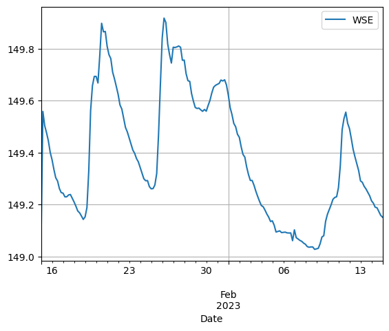

Datos de entrada

Puede descargar los datos de entrada desde este enlace:

owncloud.hatarilabs.com/s/LHpEe67q0kbYFCq

Password: Hatarilabs