Las imágenes satelitales nos brindan información sobre la superficie en base de distintas bandas, esta información viene dada por un arreglo de pixeles que constituyen la imagen a una resolución determinada. En base de combinaciones de bandas podemos decidir si un pixel representa un tipo de suelo o un tipo de cobertura, pero como hacemos para que la imagen reconozca cosas? Esto se hace mediante el uso de un nivel mayor en el análisis espacial que son los algoritmos de inteligencia artificial que son cada vez más populares y que su uso es más amigable con el usuario.
Para este tutorial hemos utilizado Python como lenguaje para el manejo de imágenes como matrices y algoritmos de Scikit-Learn para la identificación de cultivos. El tutorial también muestra herramientas interactivas de Jupyter para la selección de cultivos y la posibilidad de eliminar puntos de referencia no válidos.
Tutorial
Código
Aqui todo el código en Python utilizado en el tutorial
# Import the require libraries and images

%matplotlib notebook
import numpy as np
import matplotlib.pyplot as plt
from skimage.feature import match_template
from PIL import Image

ImagenTotal = np.asarray(Image.open('Input\OlivoTotal.png'))

# Interactive selection of points

#define empty cells
puntosinteres = []

fig = plt.figure(figsize=(9, 6))
ax = fig.add_subplot(111)
ax.imshow(ImagenTotal, cmap=plt.cm.gray)
text=ax.text(0,0, "", va="bottom", ha="left")

#interactive function that stores points clicked on the image
def onclick(event):
    tx = 'button=%d, x=%d, y=%d, xdata=%f, ydata=%f' % (event.button, event.x, event.y, event.xdata, event.ydata)
    text.set_text(tx)
    puntosinteres.append([event.xdata, event.ydata])

cid = fig.canvas.mpl_connect('button_press_event', onclick)

# amount of points clicked
len(puntosinteres)

#plot points over the image and select more if you want
fig = plt.figure(figsize=(10, 6))
ax = fig.add_subplot(111)
ax.imshow(ImagenTotal, cmap=plt.cm.gray)
ax.scatter([x[0] for x in puntosinteres],[y[1] for y in puntosinteres],c='red', marker='+', s=8)
text=ax.text(0,0, "", va="bottom", ha="left")

def onclick(event):
    tx = 'button=%d, x=%d, y=%d, xdata=%f, ydata=%f' % (event.button, event.x, event.y, event.xdata, event.ydata)
    text.set_text(tx)
    puntosinteres.append([event.xdata, event.ydata])

cid = fig.canvas.mpl_connect('button_press_event', onclick)

#show all the points of interest, please be careful to have a complete image, otherwise the model wont run
fig, ax = plt.subplots(len(puntosinteres)//6+1, 6)
i = 0
for item in puntosinteres:
    xinteres = int(item[0])
    yinteres = int(item[1])
    radio = 20
    ax[i//6,i-i//6*6].imshow(ImagenTotal)
    ax[i//6,i-i//6*6].plot(xinteres,yinteres,color='red', linestyle='dashed', marker='+',
     markerfacecolor='blue', markersize=8)
    ax[i//6,i-i//6*6].set_xlim(xinteres-radio,xinteres+radio)
    ax[i//6,i-i//6*6].set_ylim(yinteres-radio,yinteres+radio)
    ax[i//6,i-i//6*6].axis('off')
    ax[i//6,i-i//6*6].set_title(i)
    i+=1

#in case you have a wrong point or a incomplete image please uncomment the following line with the point index to delete it
#del puntosinteres[13]
len(puntosinteres)

# Match the image to the template

listaresultados = []
for punto in puntosinteres:
    xinteres = int(punto[0])
    yinteres = int(punto[1])
    radio=10
    imagenband = ImagenTotal[:,:,0]
    templateband = ImagenTotal[yinteres-radio:yinteres+radio,xinteres-radio:xinteres+radio,0]
    result= match_template(imagenband, templateband)
    result = np.where(result>0.85)
    listaresultados.append(result)

# Plot interpreted points over the image

from itertools import cycle
cycol = cycle('bgrcmk')

fig = plt.figure(figsize=(10, 8))
ax = fig.add_subplot(111)

i = 1
for lista in listaresultados:
    ax.plot(lista[1],lista[0], '.', linewidth=0, markerfacecolor=next(cycol), label=i)
    i+=1
ax.legend(loc='upper center', bbox_to_anchor=(0.5, -0.05),
          fancybox=True, shadow=True, ncol=5)
ax.imshow(ImagenTotal[radio:-radio,radio:-radio,:])

# Cluster analisys with Birch algorithm

datalist = [np.asarray(pares).T for pares in listaresultados]
print(len(datalist))
datalist = np.vstack(datalist)
print(datalist)

from sklearn.cluster import Birch
brc = Birch(branching_factor=10000, n_clusters=None, threshold=10, compute_labels=True)
brc.fit(datalist)
puntosbirch = brc.subcluster_centers_
fig = plt.figure(figsize=(10, 8))
ax = fig.add_subplot(111)
ax.scatter(puntosbirch[:,[1]],puntosbirch[:,[0]], marker='+',color='red')
ax.imshow(ImagenTotal[radio:-radio,radio:-radio,:])

len(puntosbirch)
Datos de entrada
Descargue los datos de entrada de este enlace.